uint8 and uint16 are most common for images from light microscopes. float32 and float64 are common during image processing.
Coordinate system
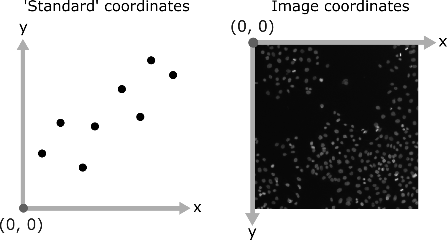
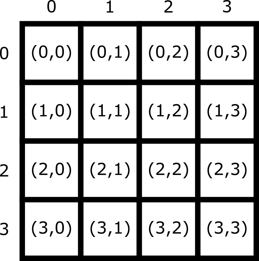
For 2d images, y is the first coordinate
For 3d images, z is the first coordinate
Handedness of the coordinate system
napari v0.6.0 and later use a right-handed 3D coordinate system by default.
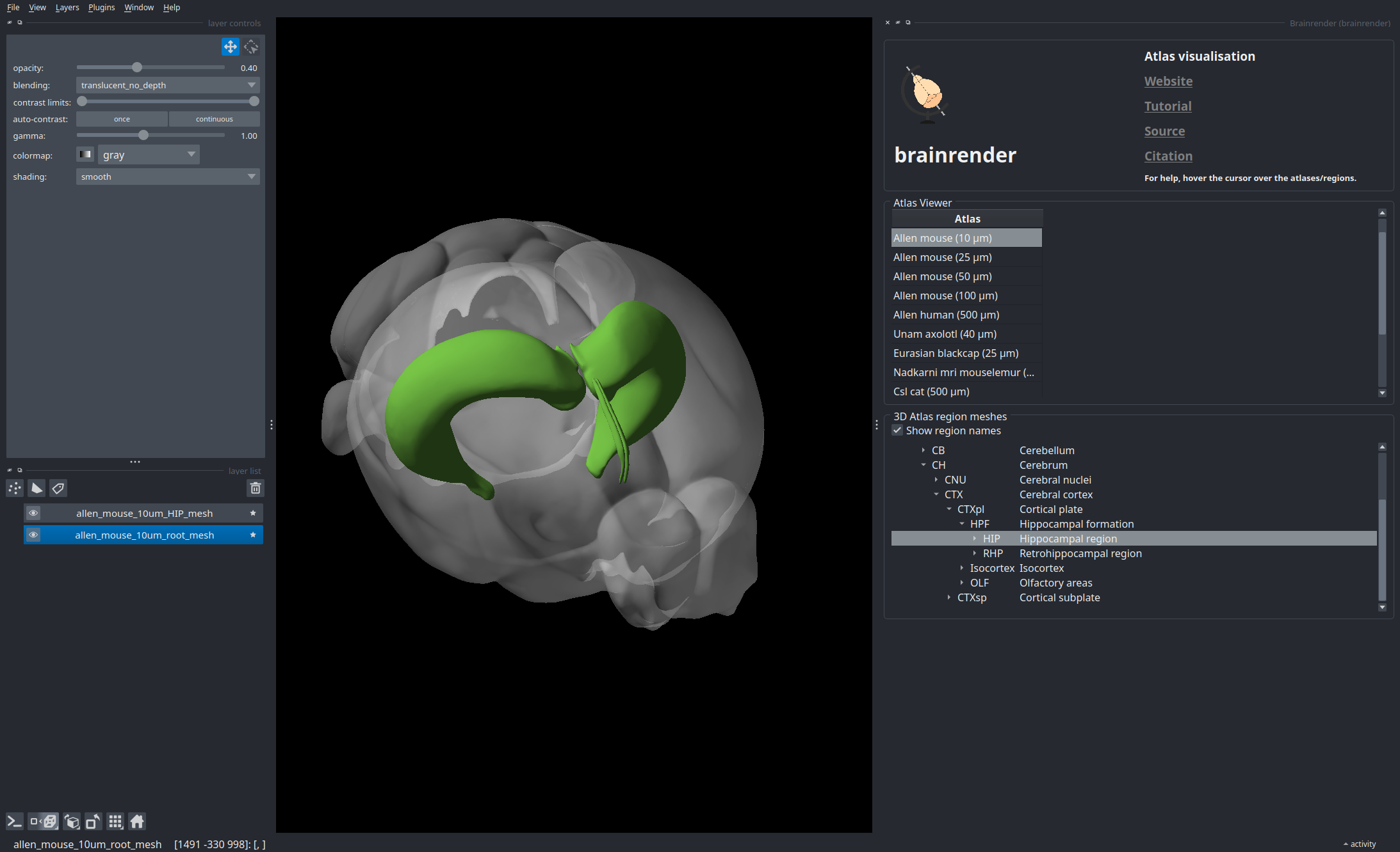
Some BrainGlobe tools (in particular brainrender) expect a left-handed system.
To change to a left-handed system:
Right-click the Toggle 2D/3D view button in the bottom-left corner.
Select the pre-0.6.0 default: away, down, right.
https://napari.org/stable/guides/axis-names.html
Axis names
napari v0.7.0 and later use a negative numbers as axis names by default.
think of it like Python indexing: in a 3D image, index 0 is index -3.
Visualise the origin and axis direction with View > Axes > Axes visible
Demo: handedness and axis names
Key points
Digital images are made of pixels
Digital images store these pixels as arrays of numbers
Napari (and Python more widely) use NumPy arrays to store images - these have a shape and dtype
Most images are 8-bit or 16-bit unsigned integer
Images use a coordinate system with (0,0) at the top left, x increasing to the right, and y increasing down
BrainGlobe conventions (for reference)
BrainGlobe’s napari plugins work in pixel coordinates (for now)
brainrender displays in a left-handed coordinate system
this can look like a LR flip bug
Processing images
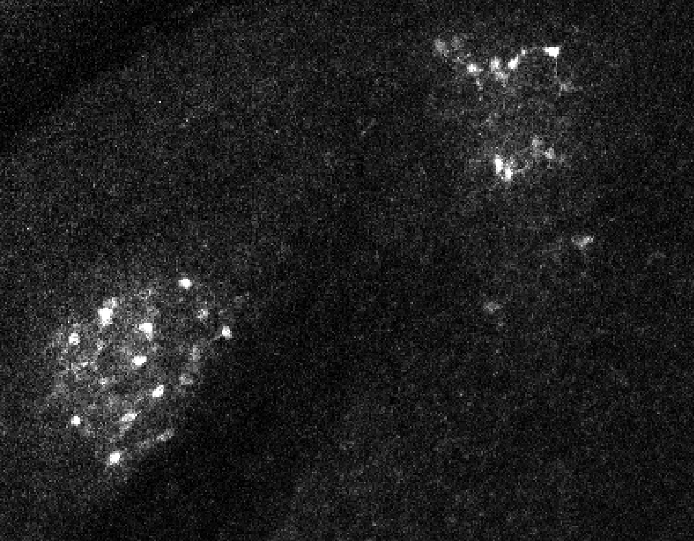
Now we understand what an image is, and how to look at it in napari, we can start measuring things! But we need to find (“segment”) “things” first!
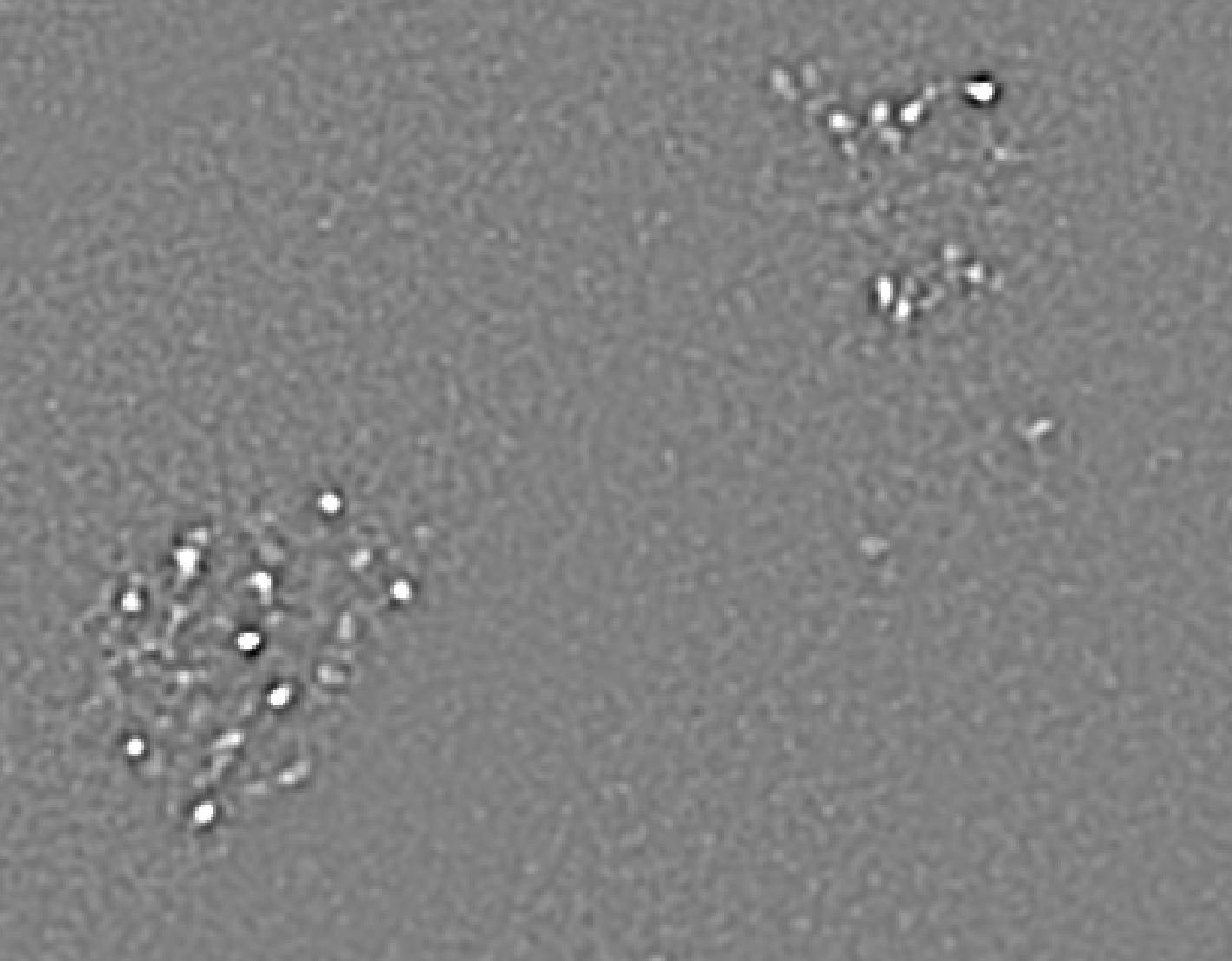
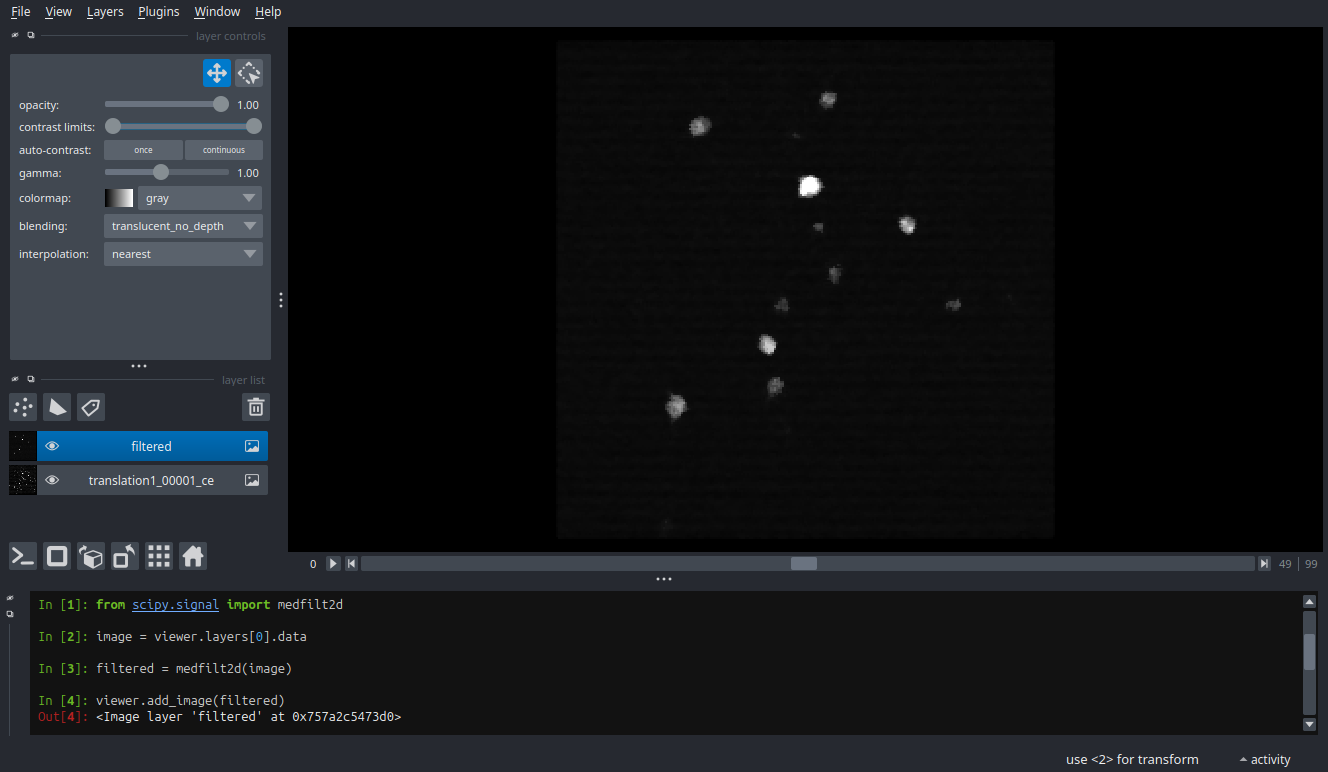
Reduce noise with a median filter
from scipy.signal import medfilt2dimage = viewer.layers[0].datafiltered = medfilt2d(image)viewer.add_image(filtered)
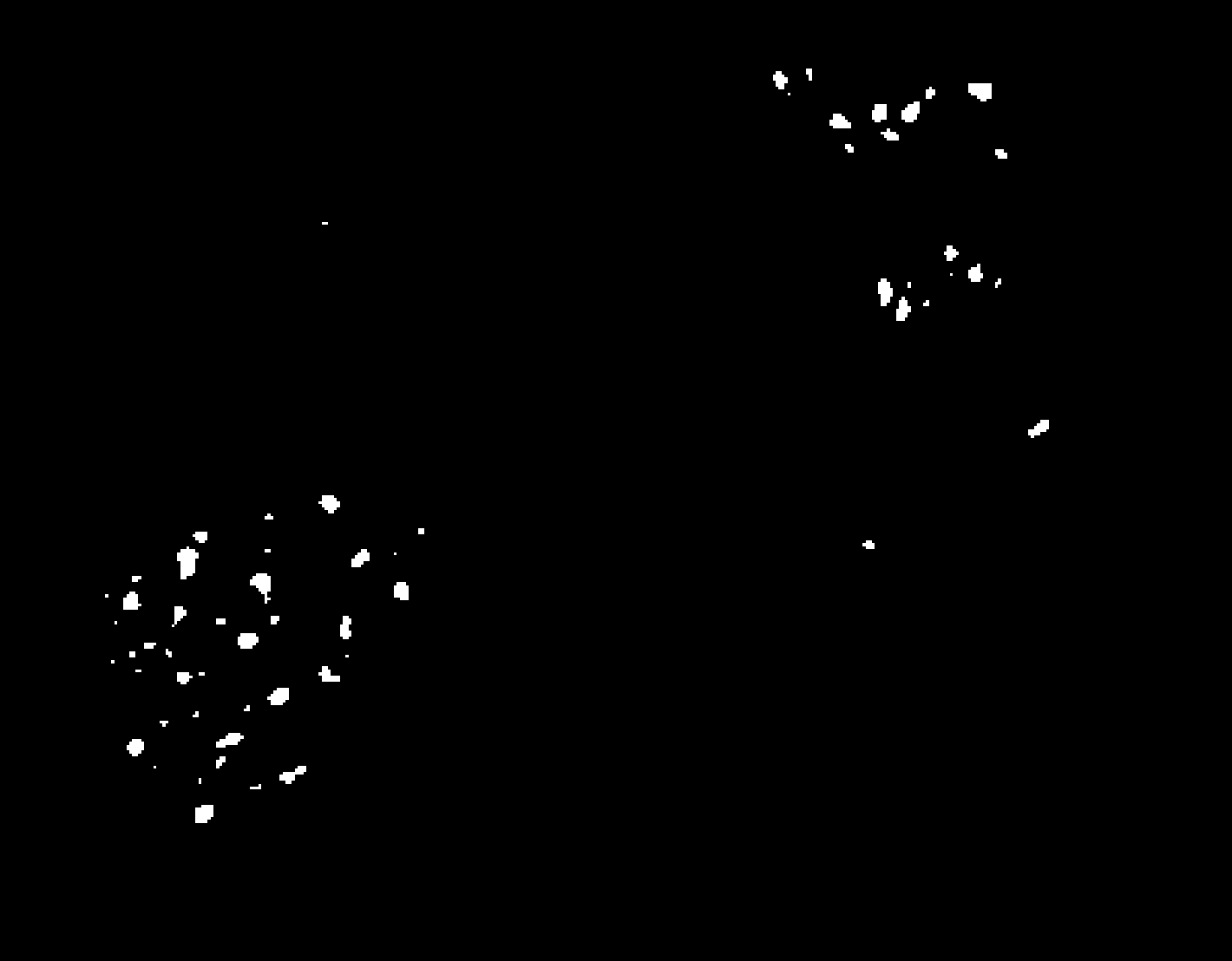
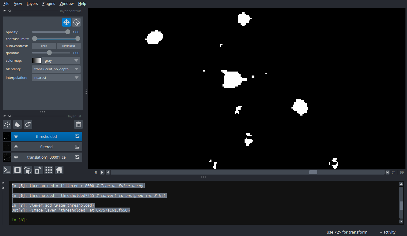
Isolate neurons with a threshold
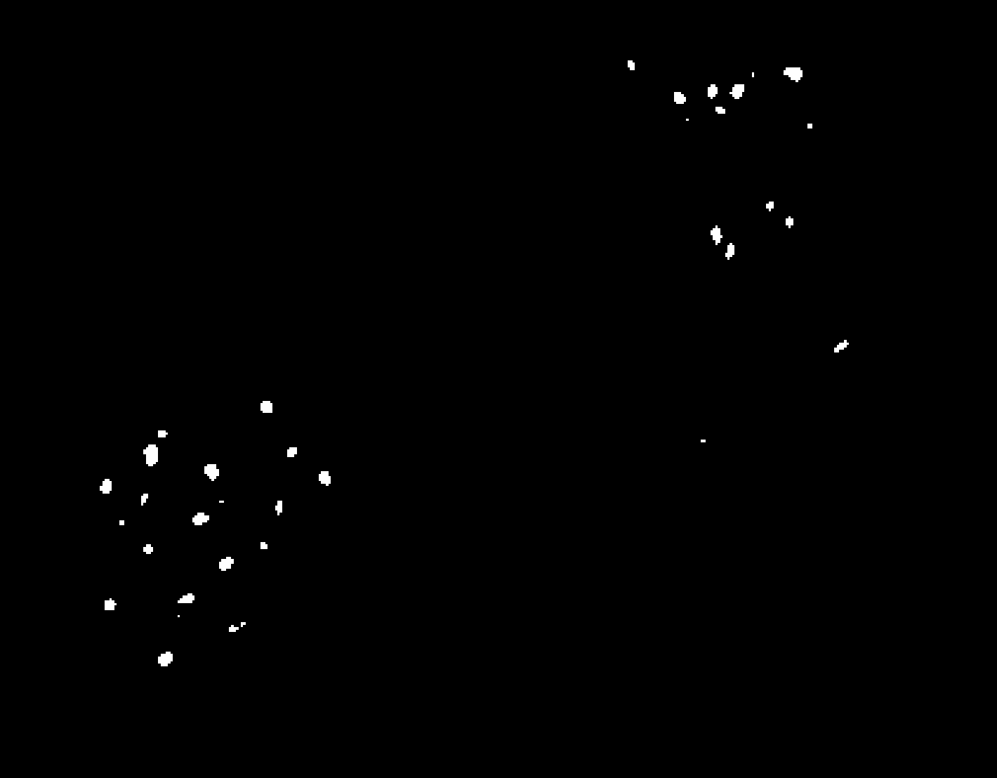
Example of “semantic” segmentation
thresholded = filtered >8000# True or False arrayviewer.add_image(thresholded)
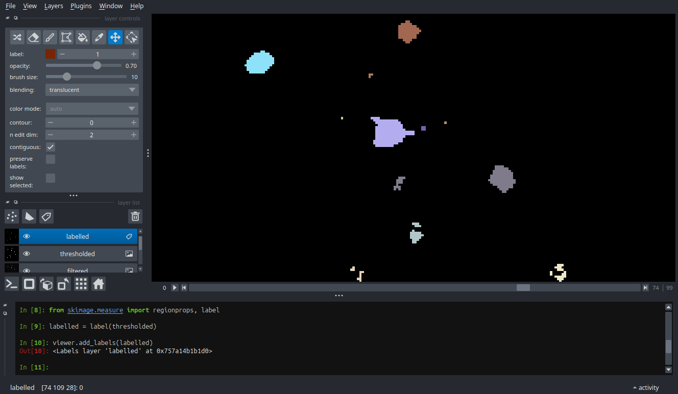
Label each neuron with a number
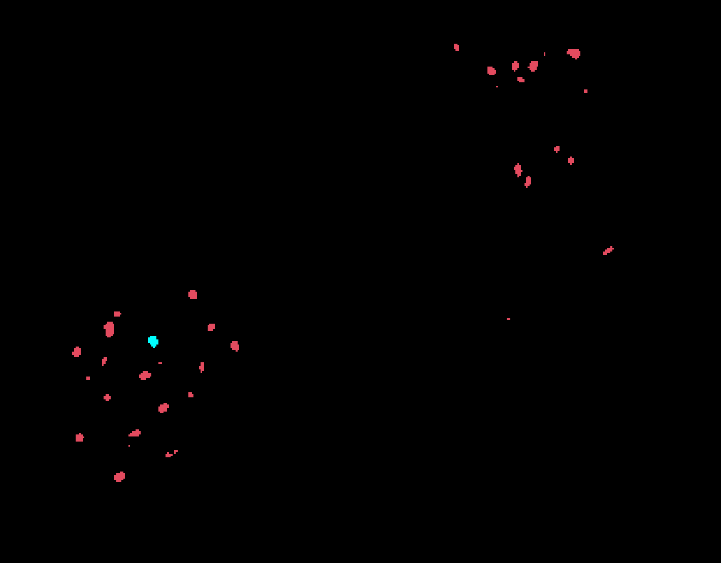
Example of “instance” segmentation
from skimage.measure import regionprops, labellabelled = label(thresholded)viewer.add_labels(labelled)
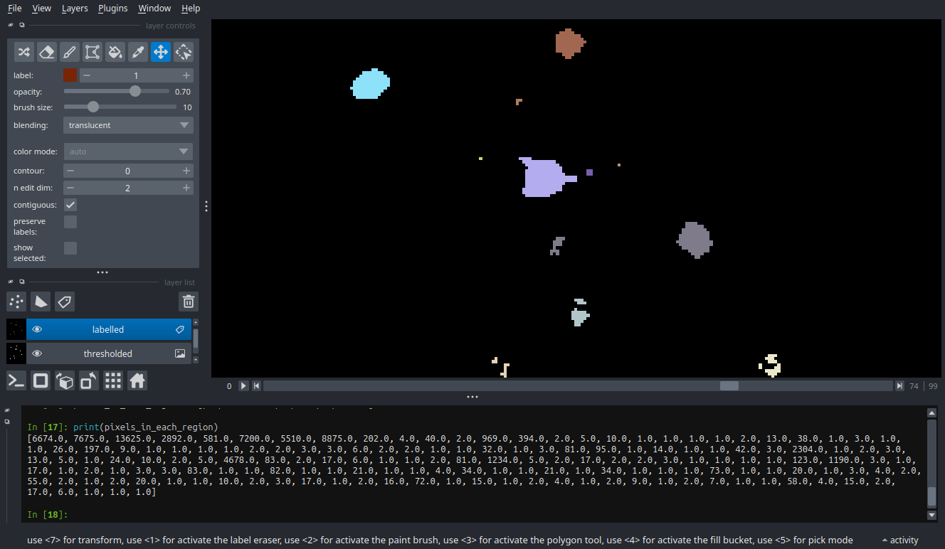
Pixels in each neuron
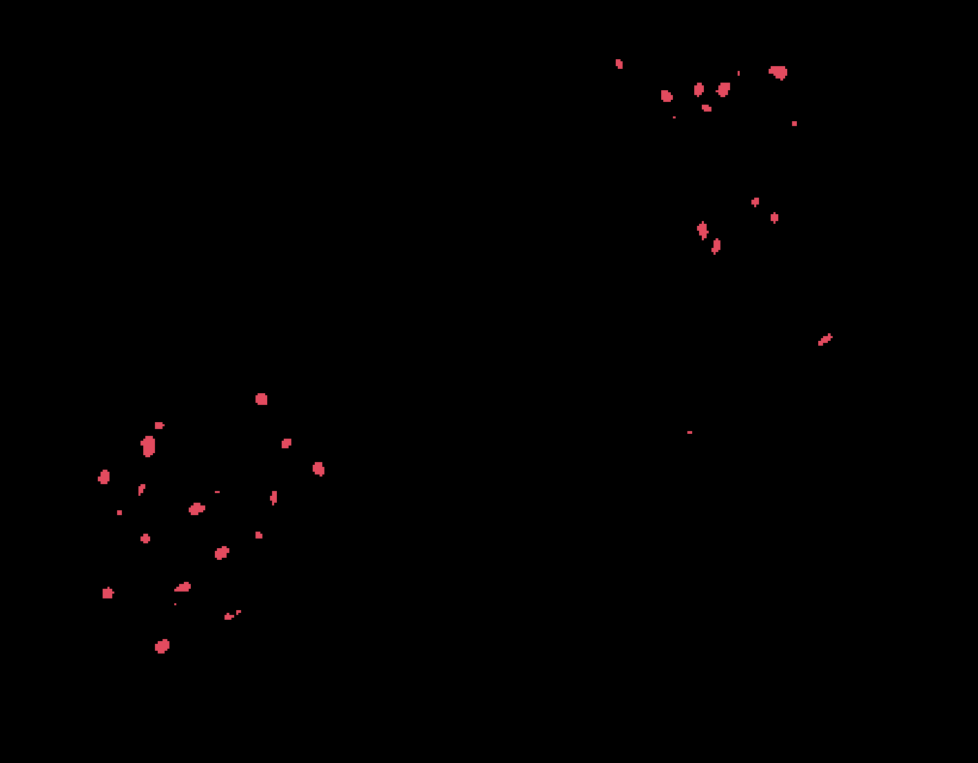
properties = regionprops(labelled)pixels_in_each_region = [prop.area for prop in properties]print(pixels_in_each_region)
Key points
Segmentation can be broadly split into ‘semantic segmentation’ (e.g. neuron vs background) and ‘instance segmentation’ (e.g. individual neuron).
Segmentations are represented in the computer in the same way as images, but pixels represent an abstraction, rather than light intensity.
Napari uses “Labels” layers for segmentations.
Segmentation is helpful for analysis.
BrainGlobe
Background
Our goal at the BrainGlobe Initiative is to accelerate progress in neuroscience by providing a set of interoperable tools – and building a community – for computational neuroanatomy.
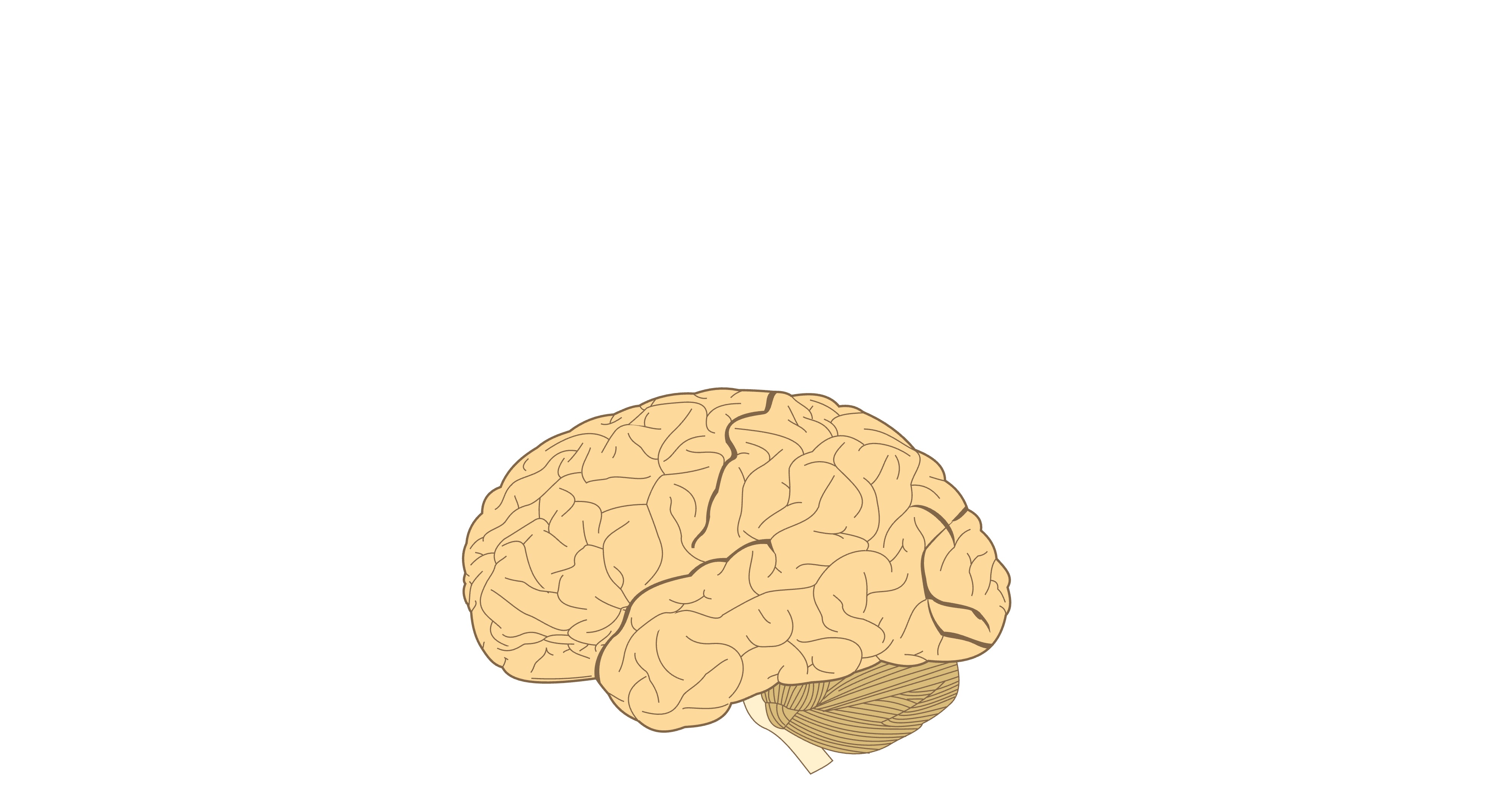
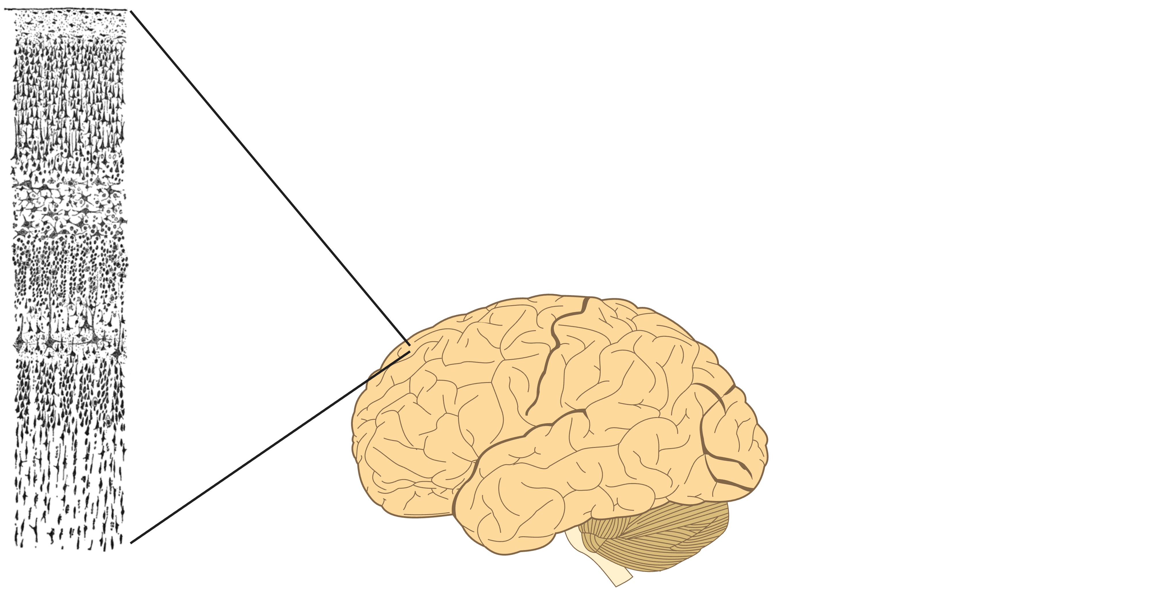
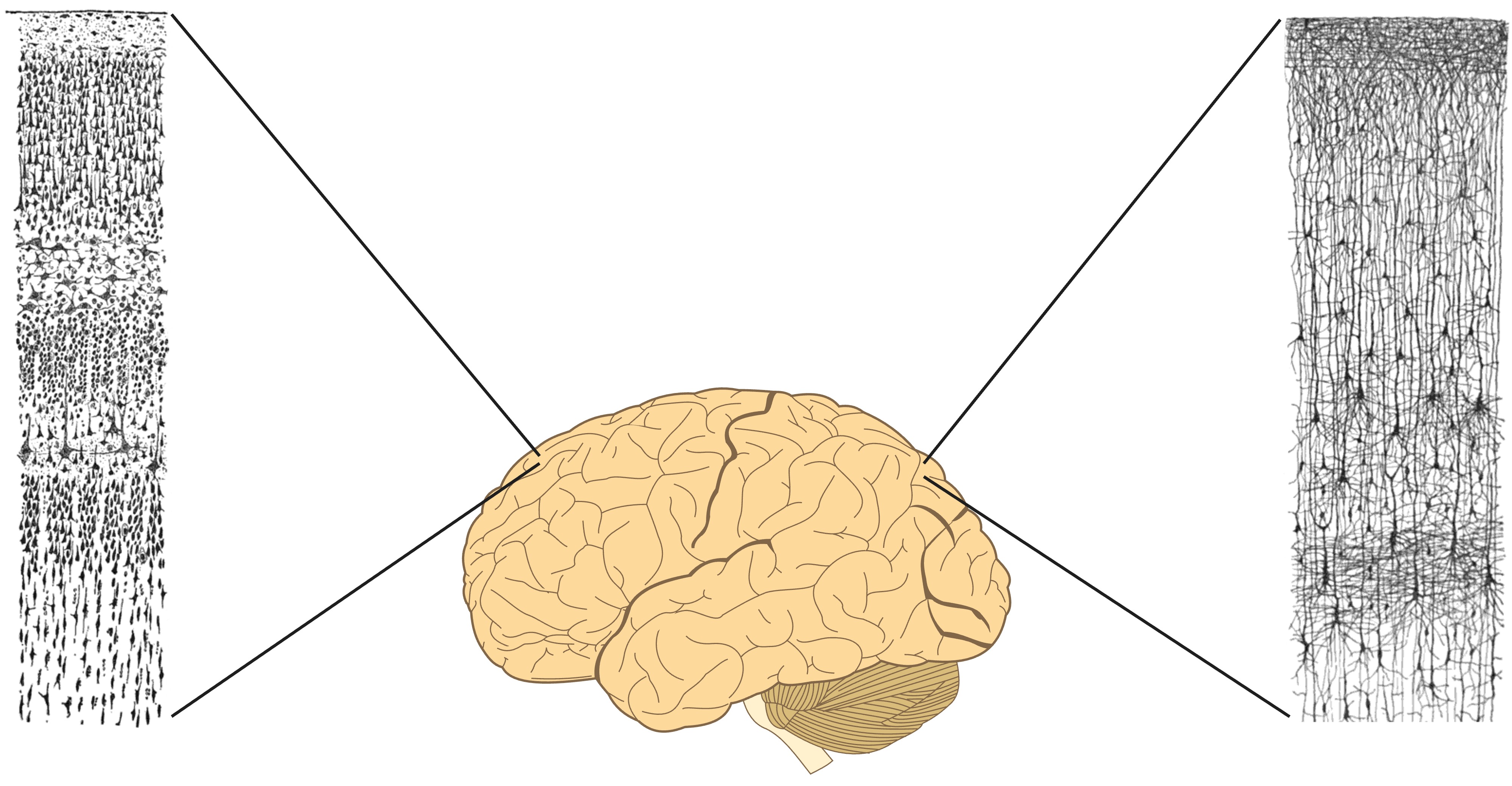
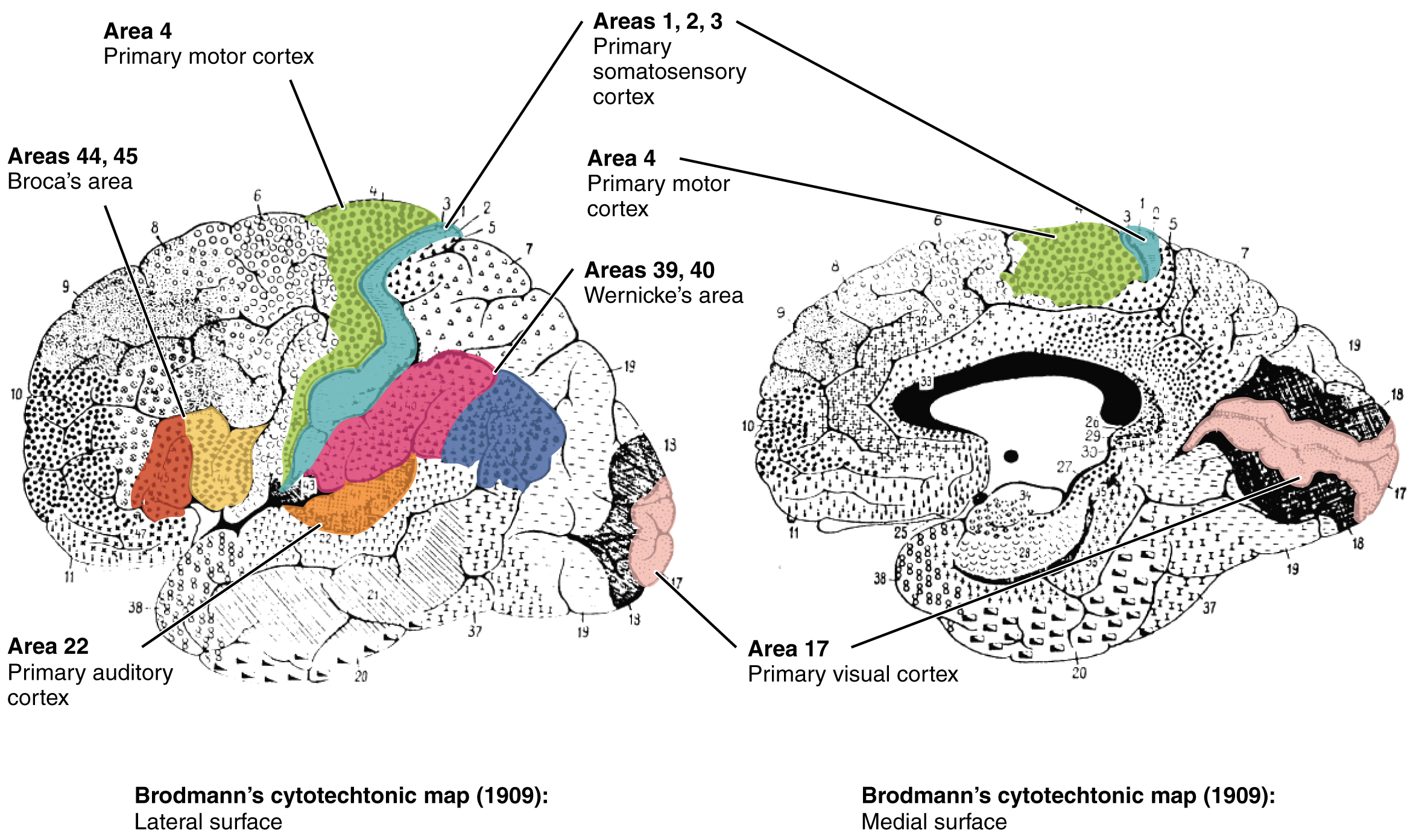
Understanding the brain
Understanding the brain
Understanding the brain
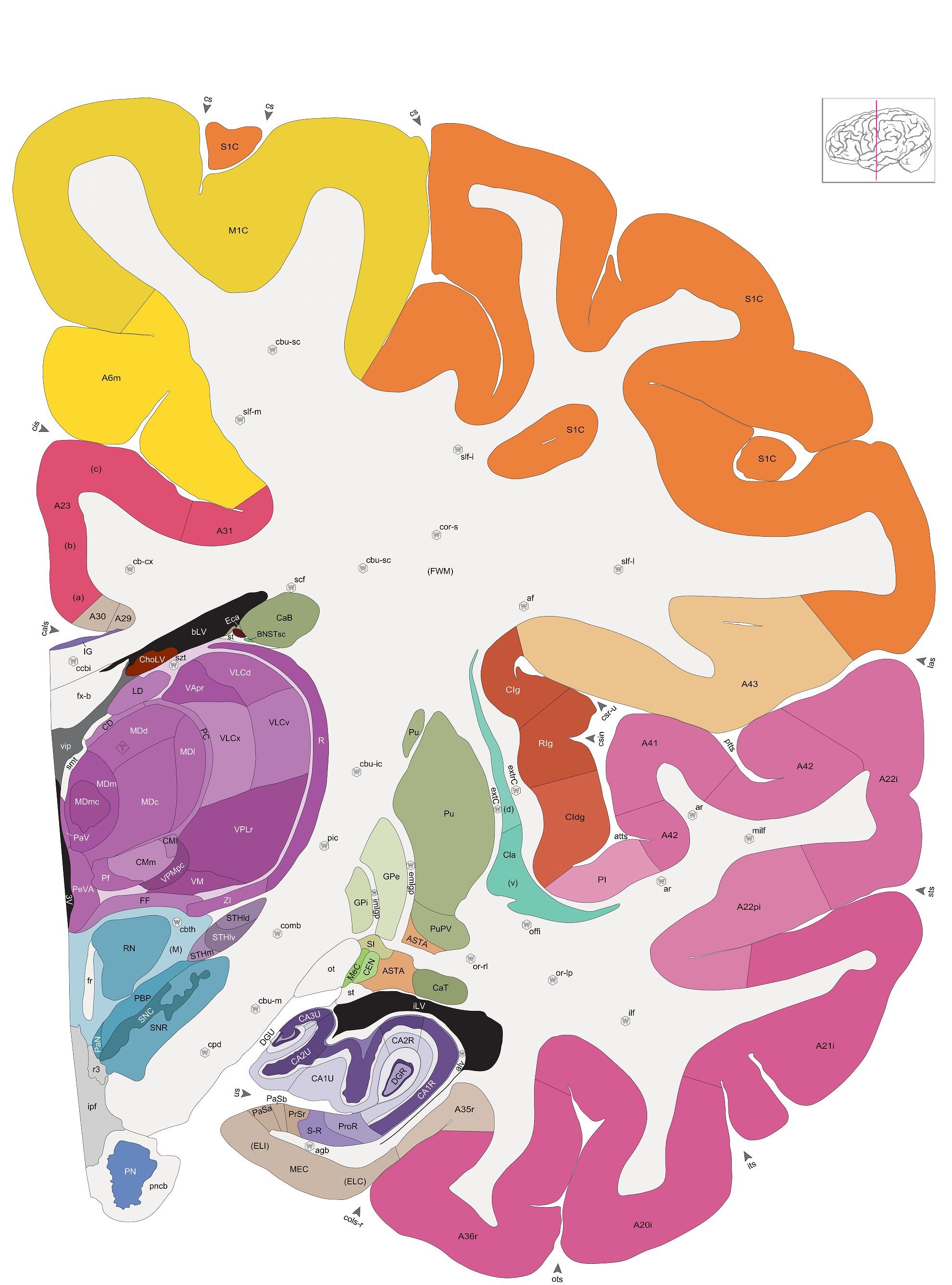
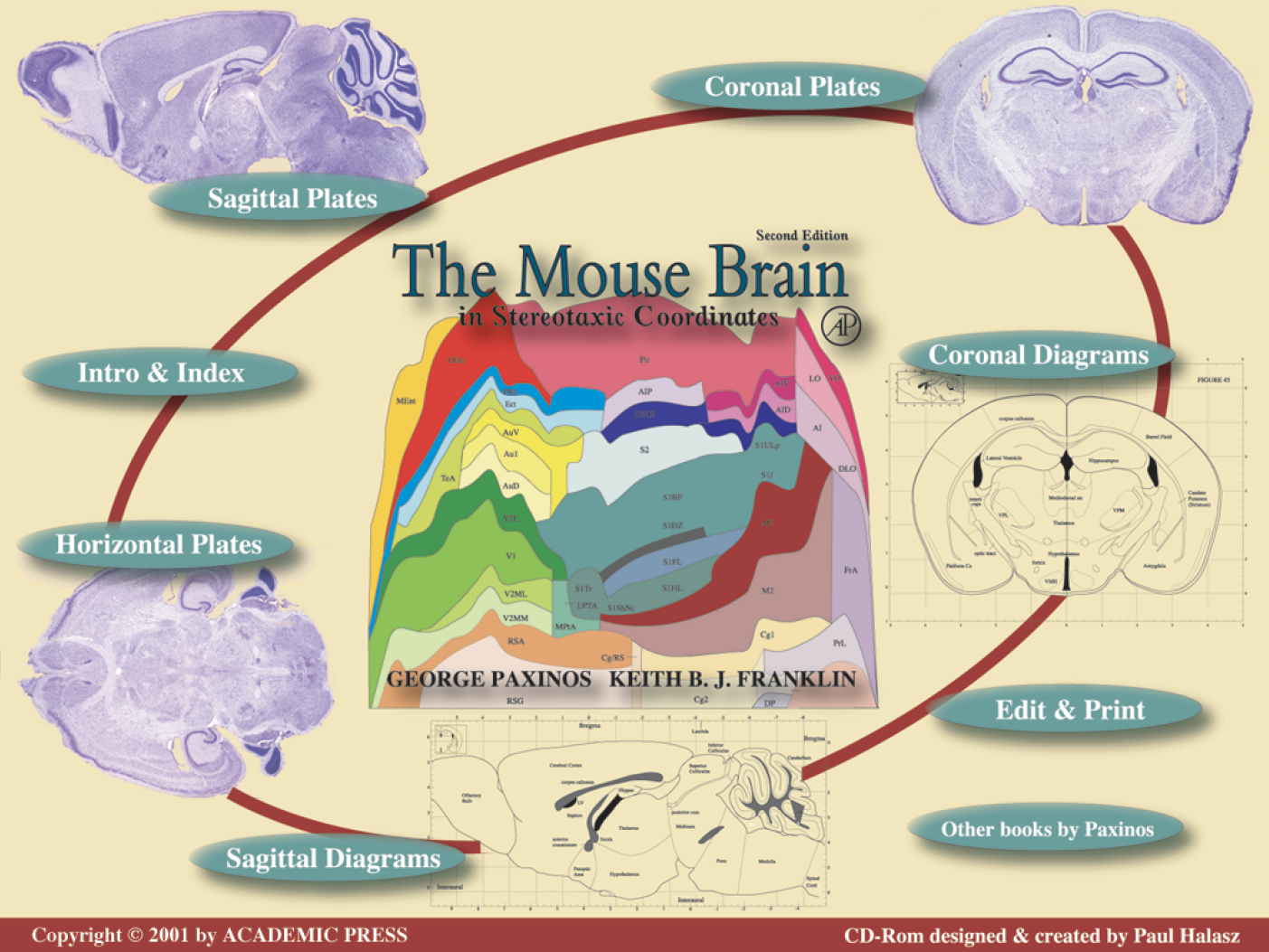
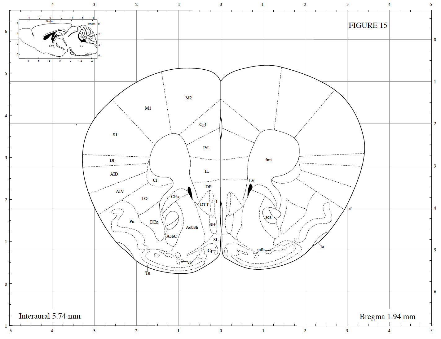
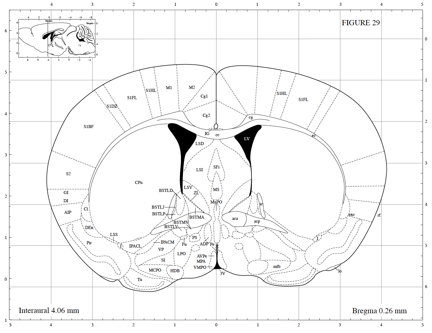
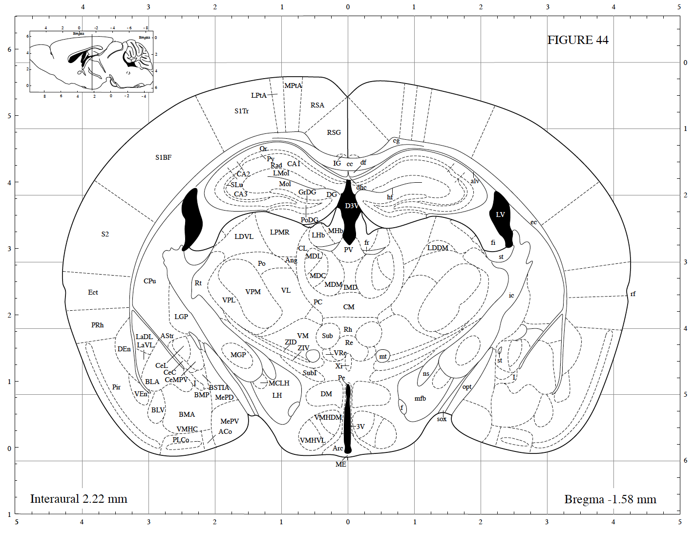
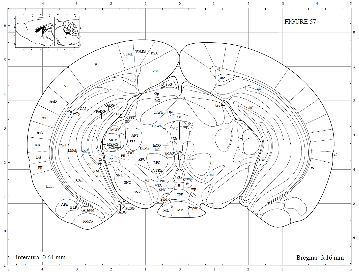
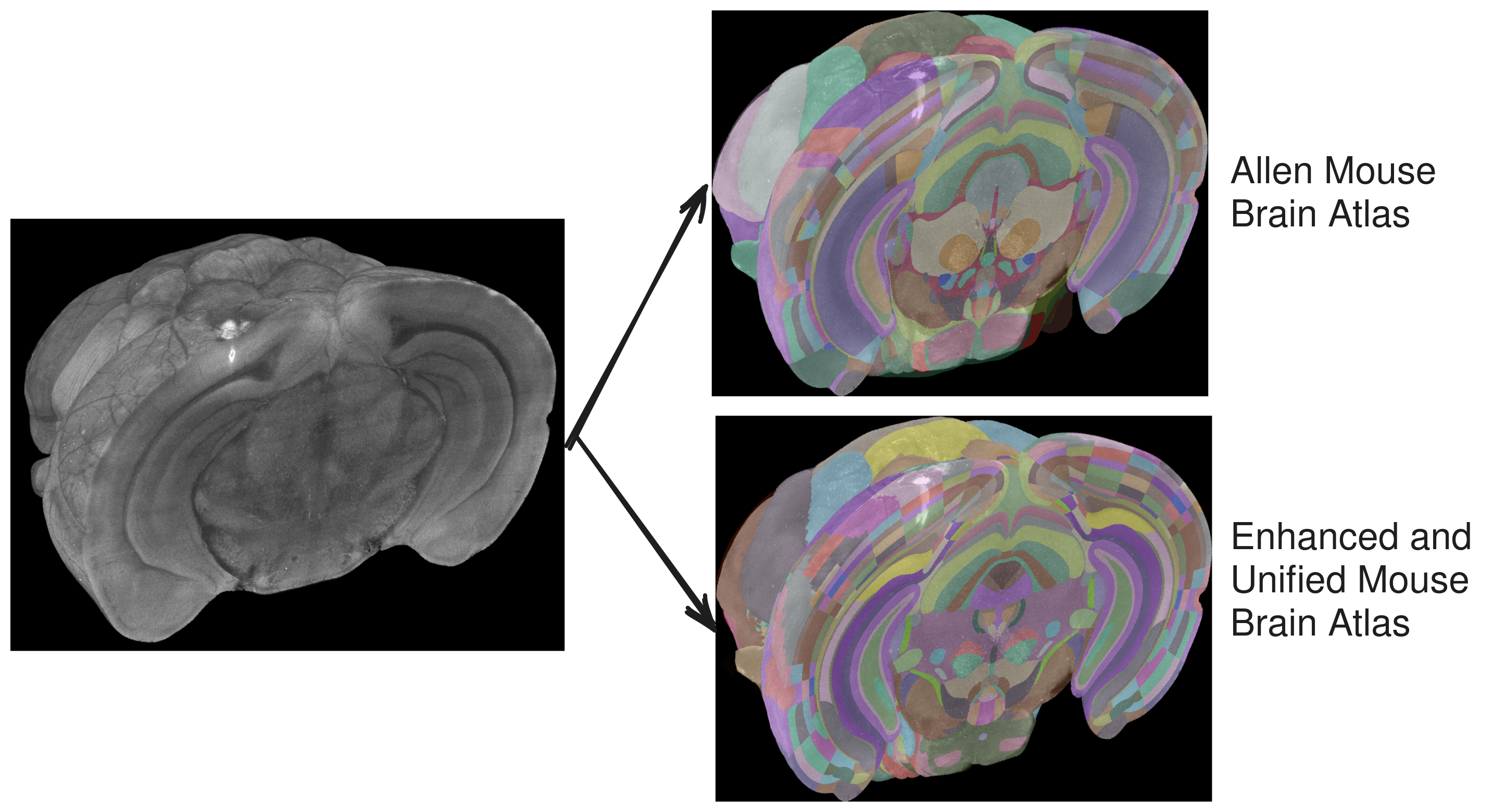
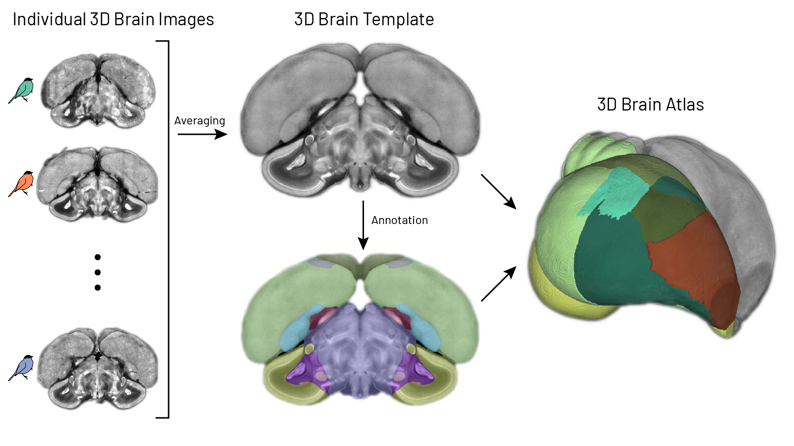
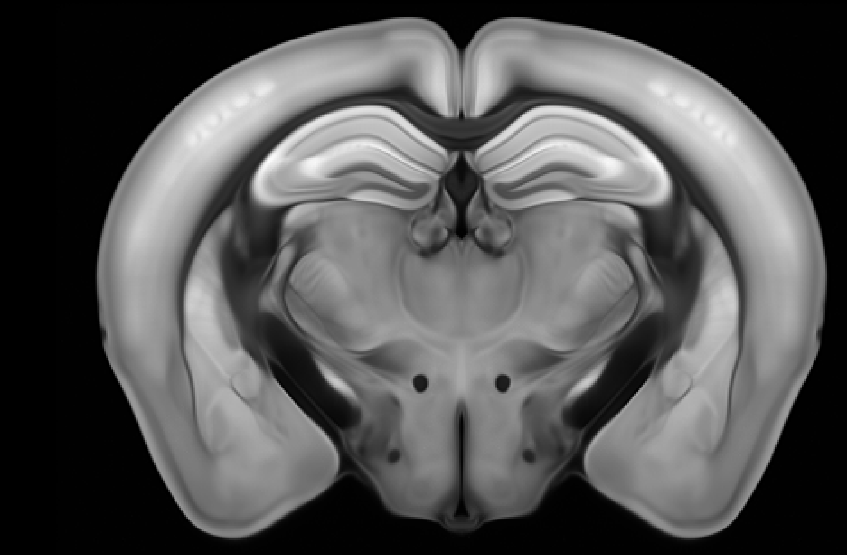
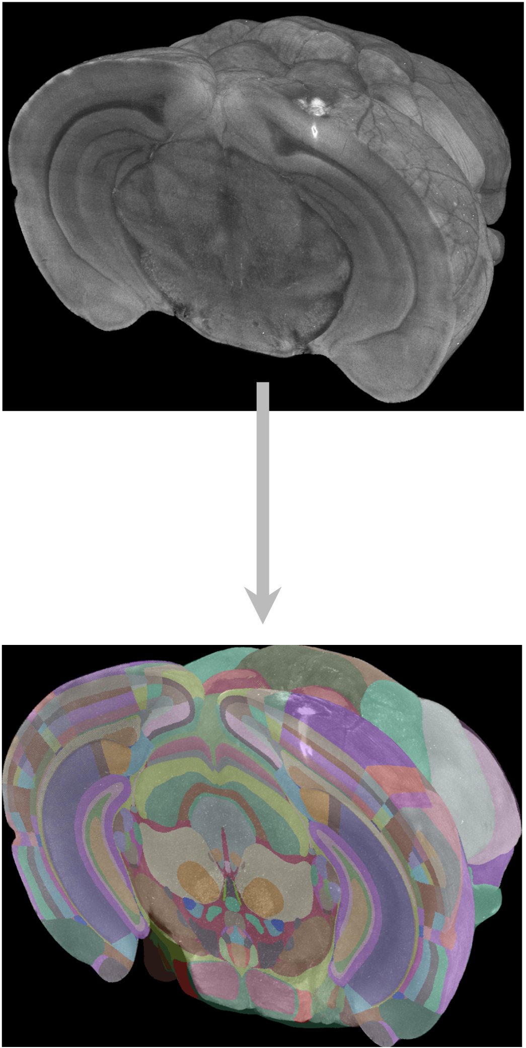
Brain atlases
Brain atlases
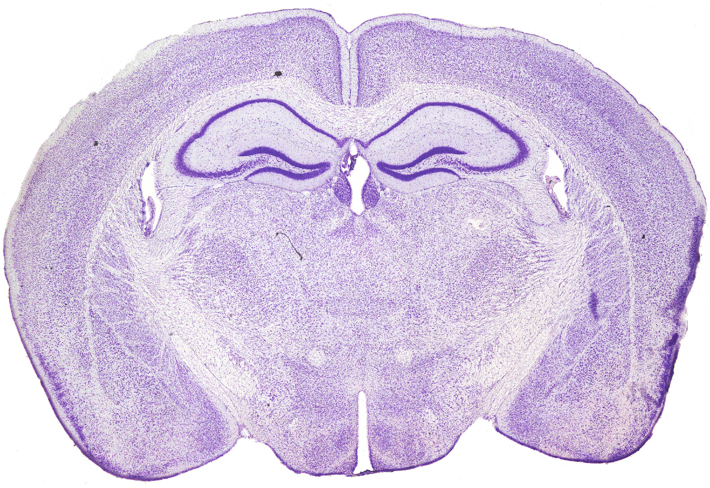
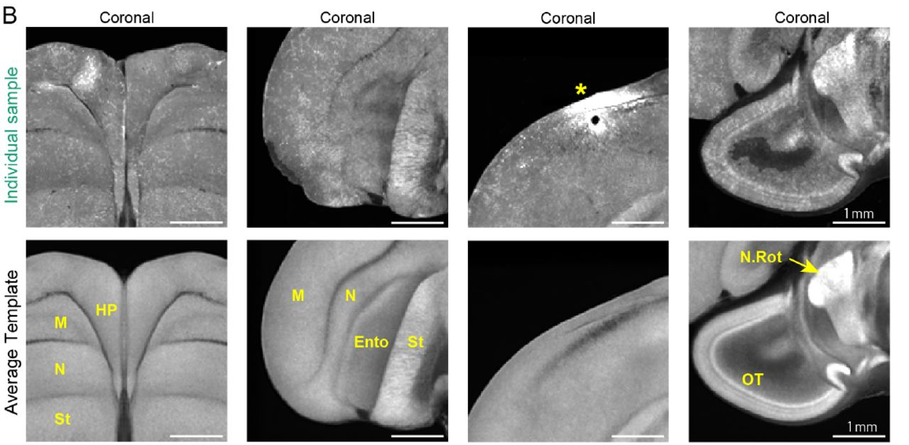
Template
Annotation
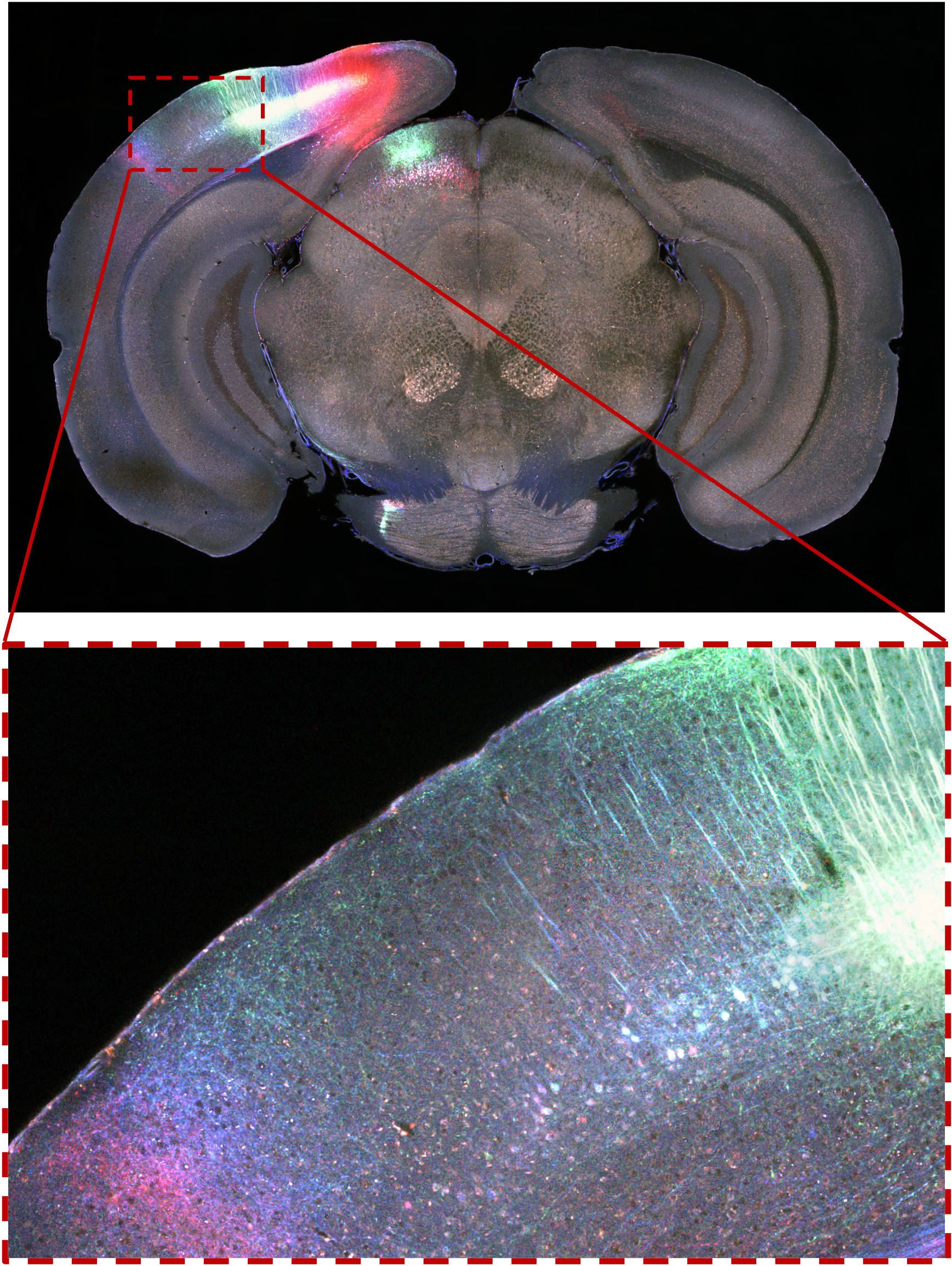
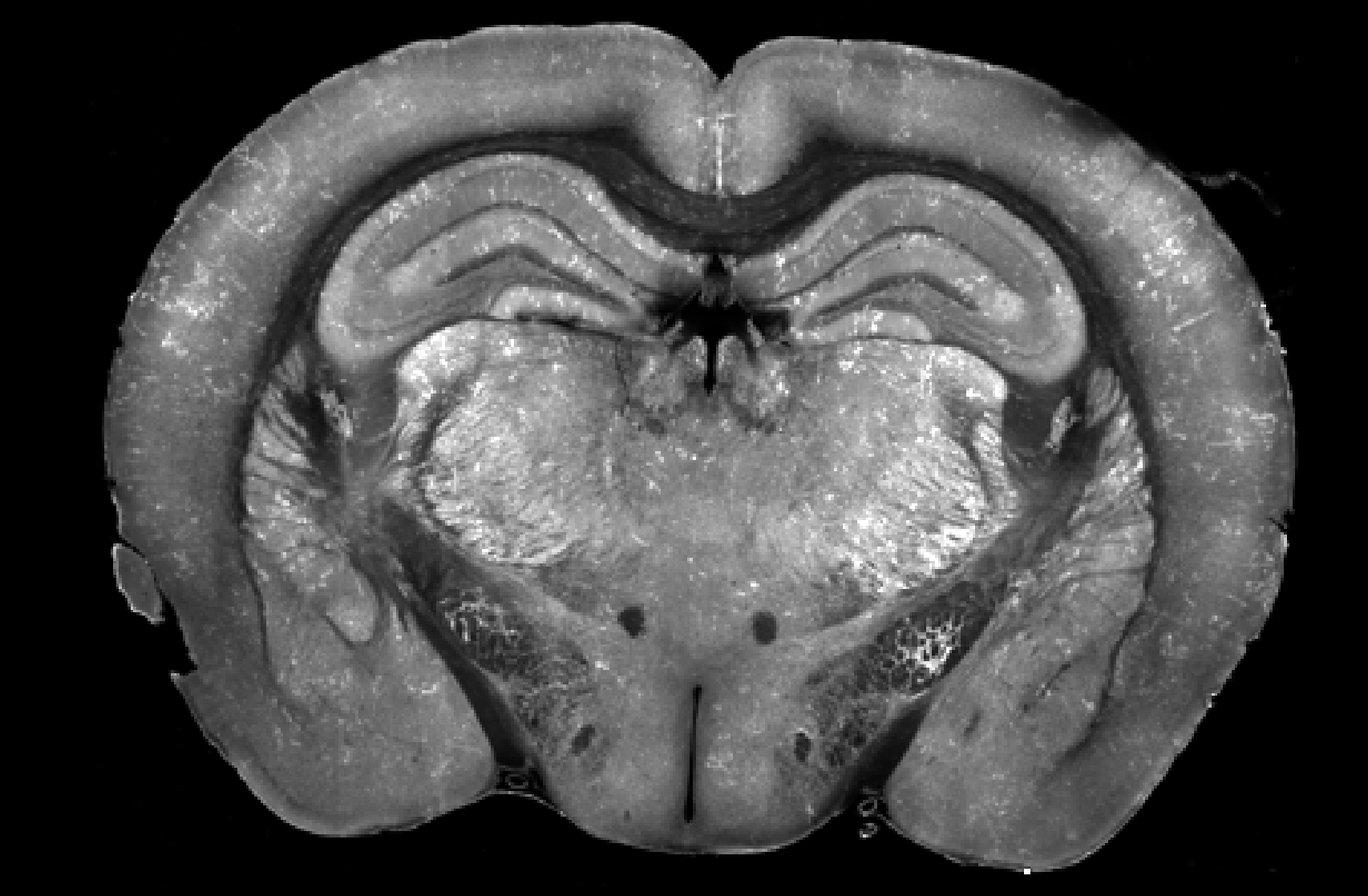
Histology
Histology
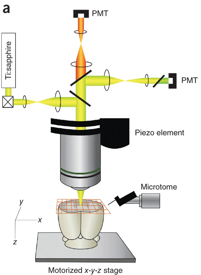
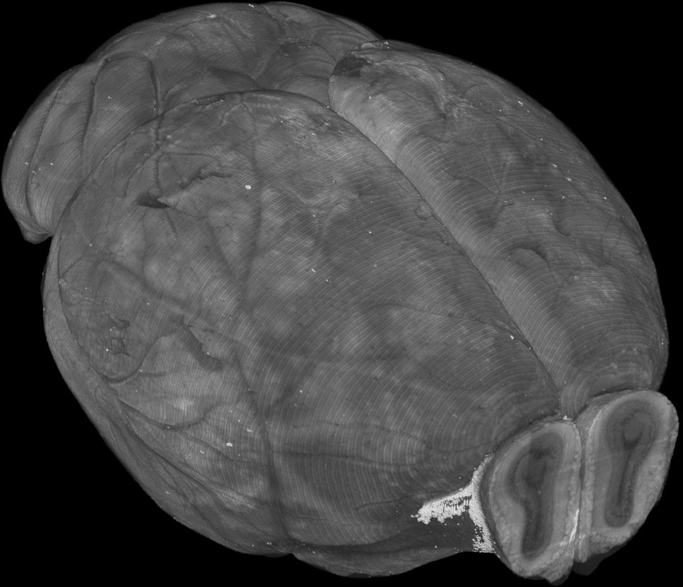
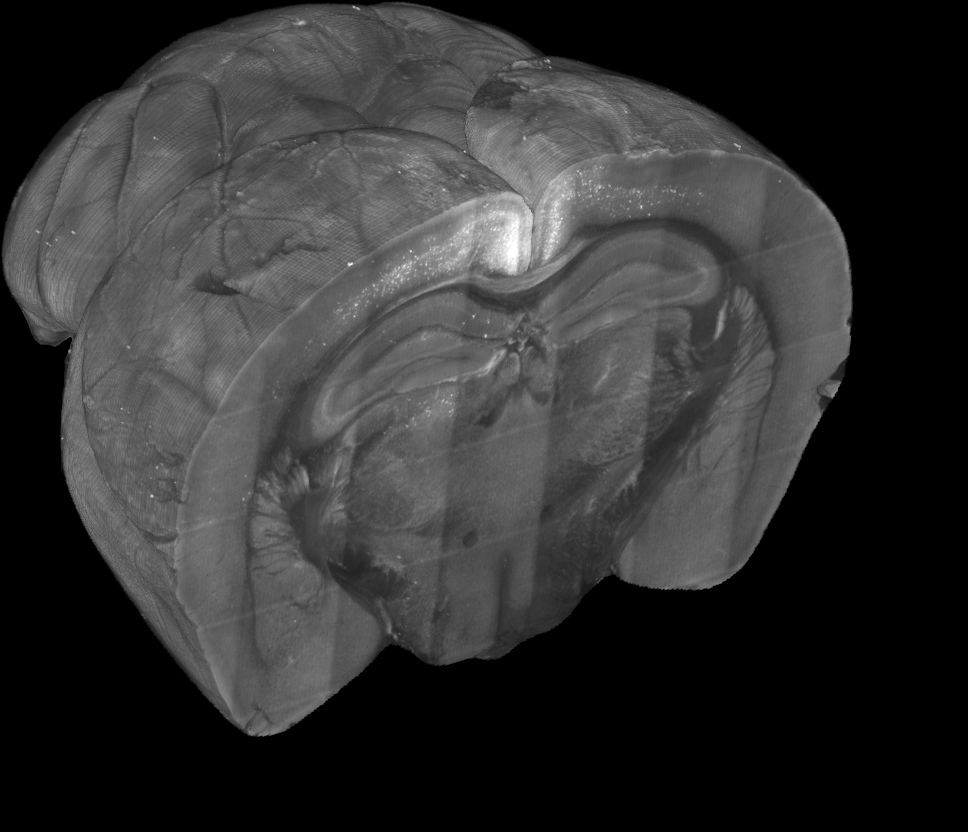
Serial two-photon tomography
Serial two-photon tomography
Serial two-photon tomography
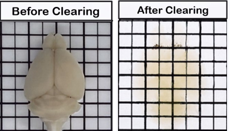
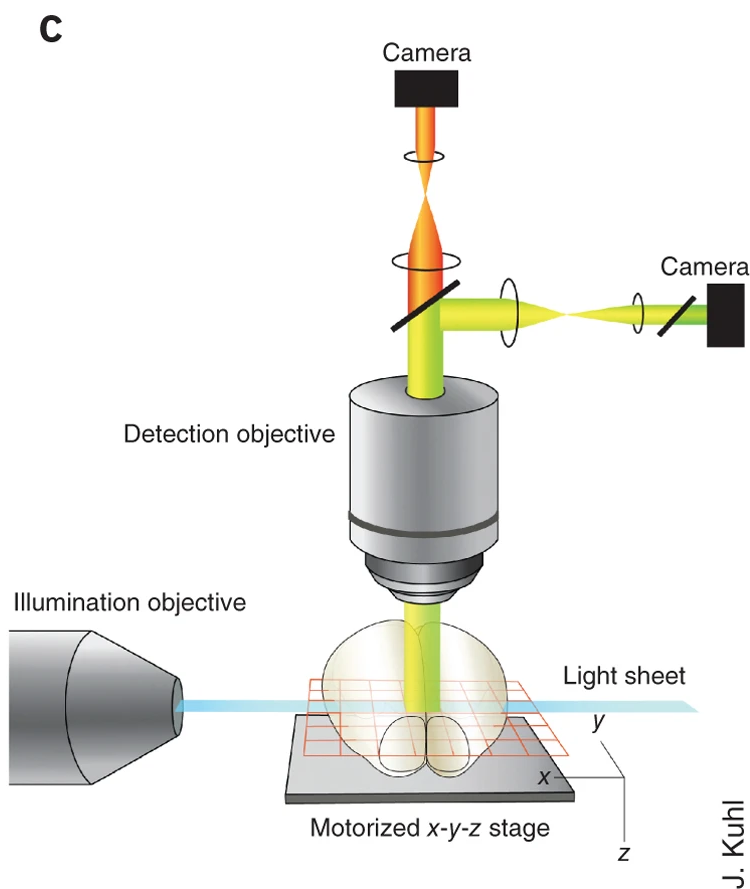
Light sheet fluorescence microscopy
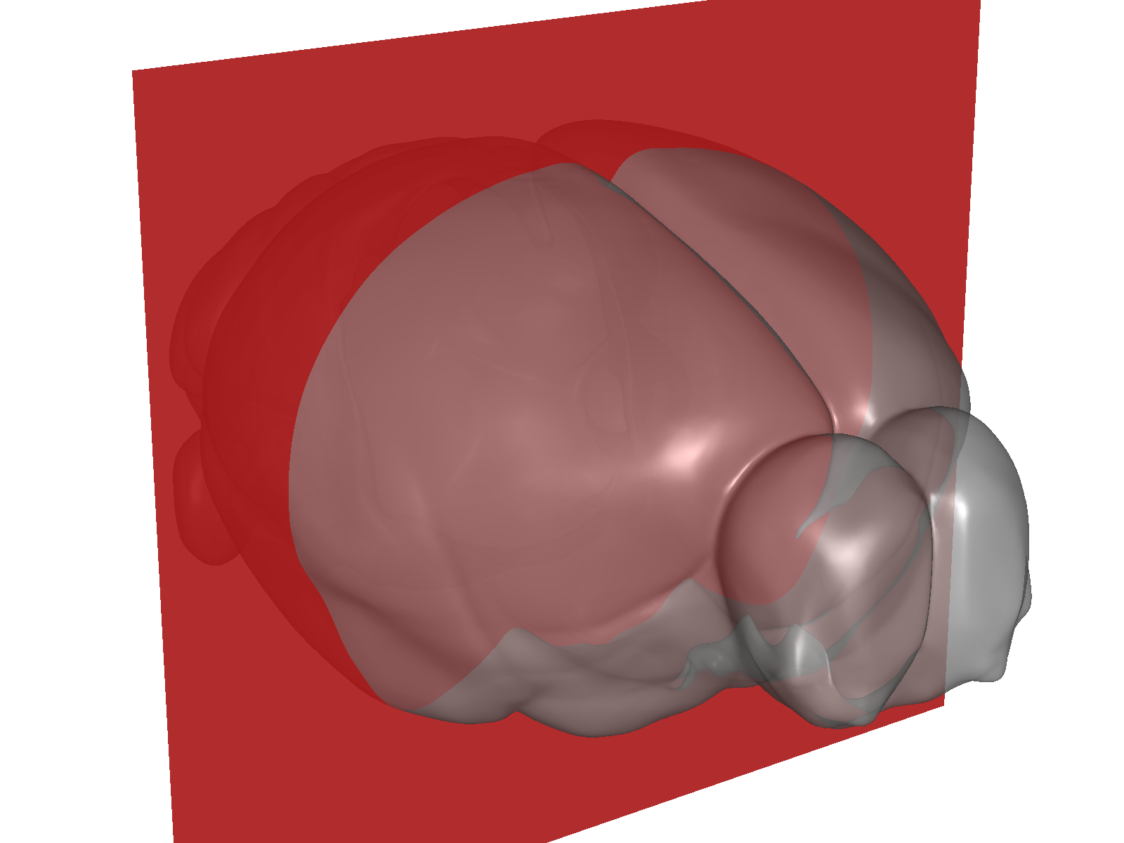
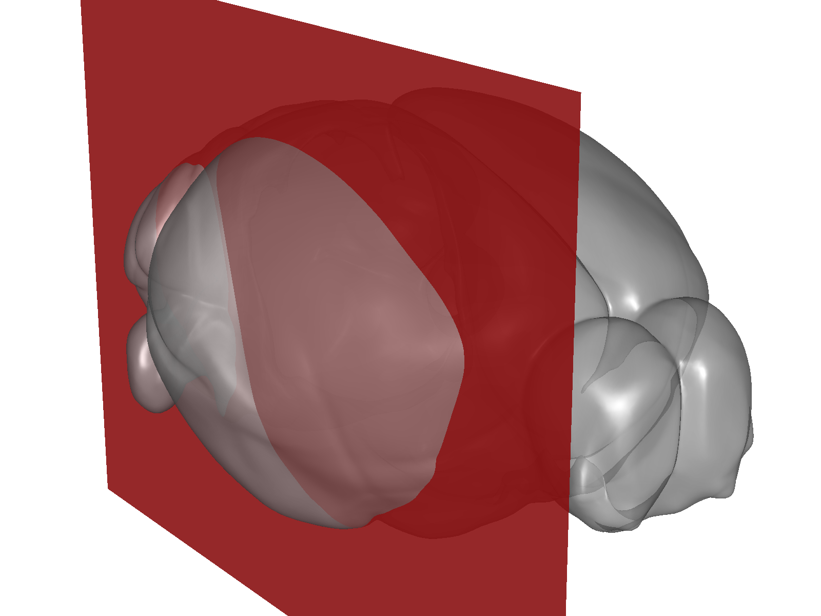
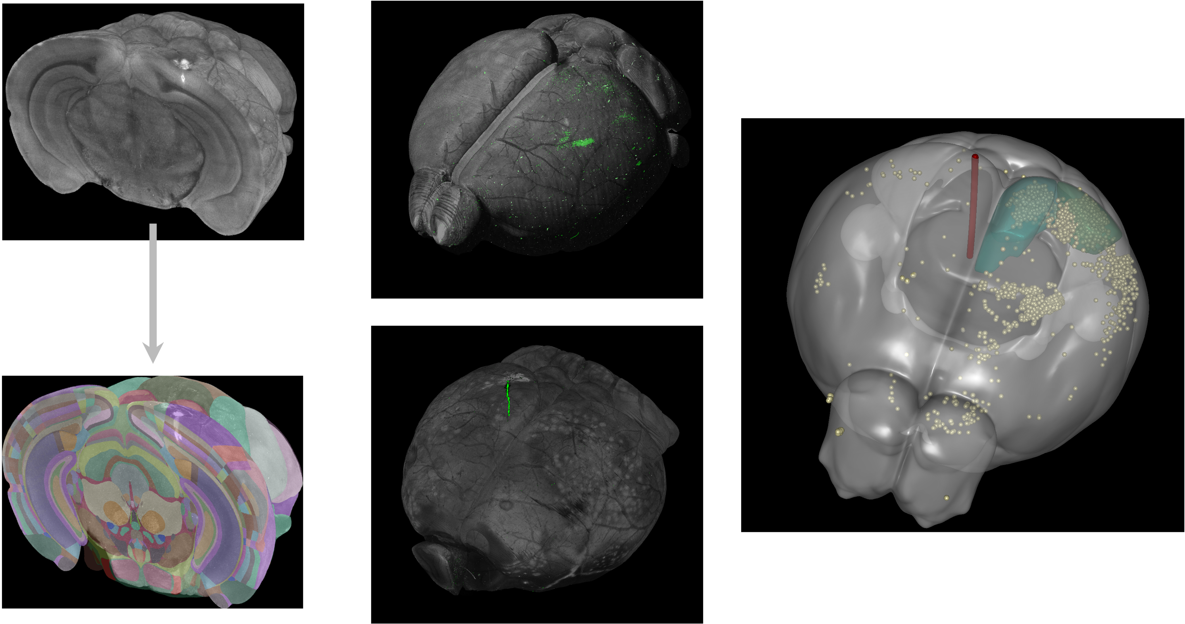
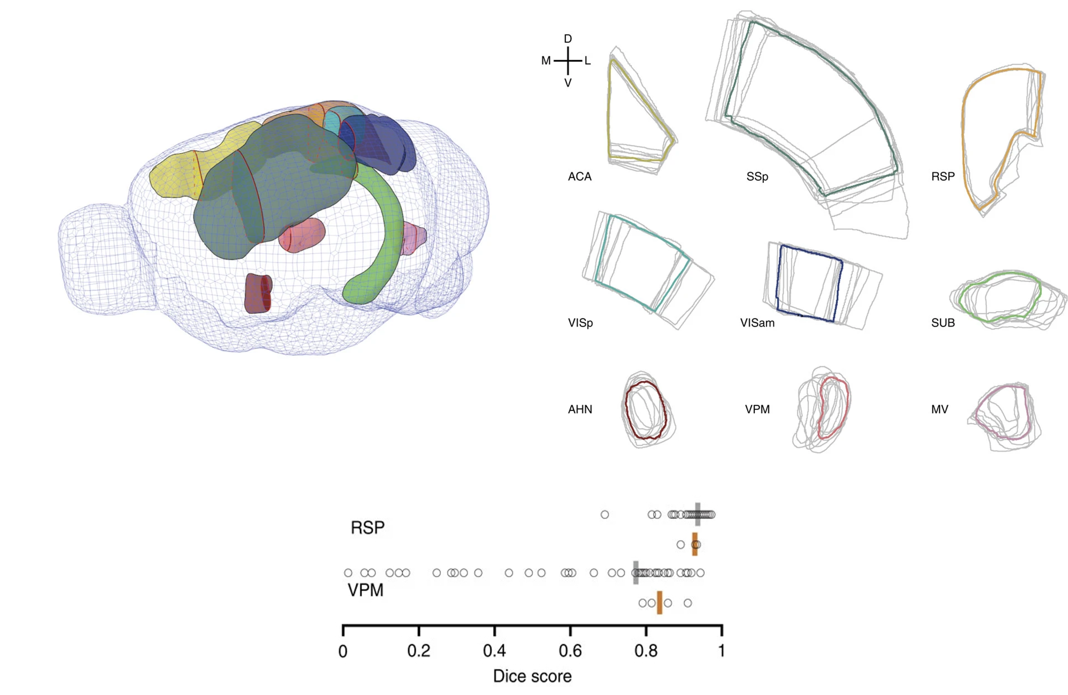
3D atlases
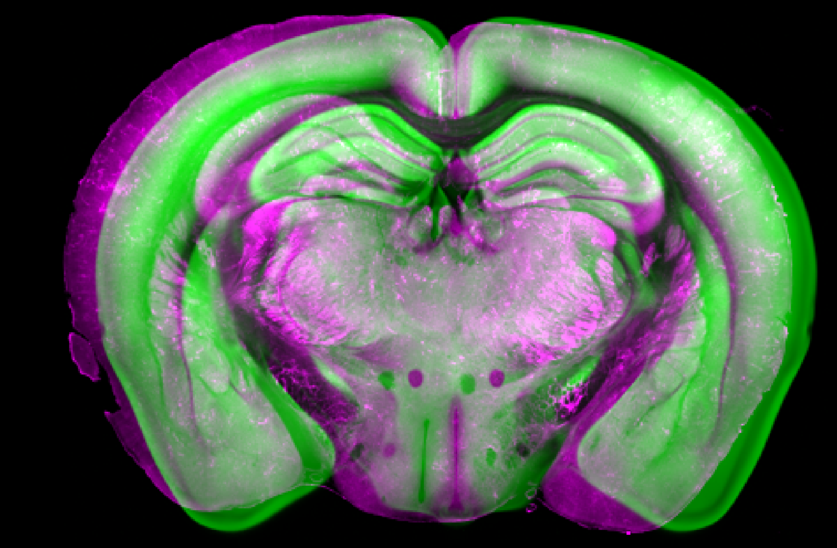
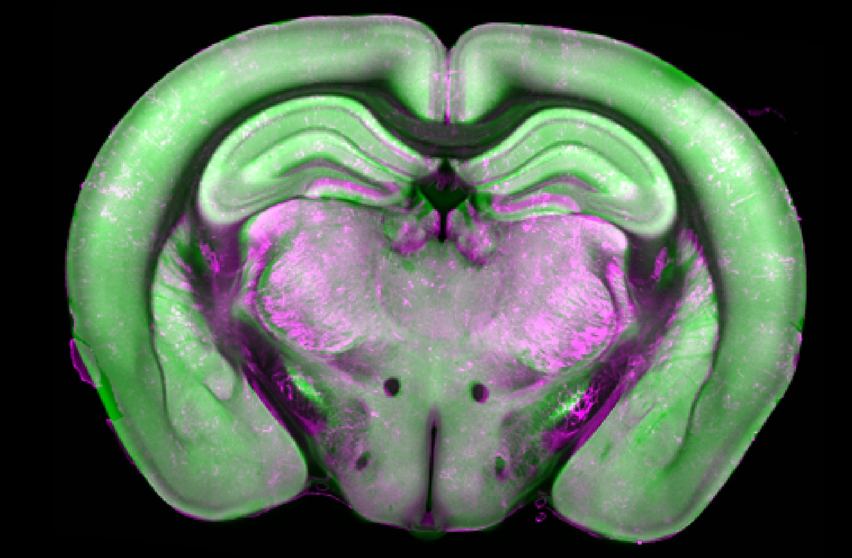
Alignment
What was needed?
A platform that enabled the community to:
Build tools for whole-brain microscopy data analysis.
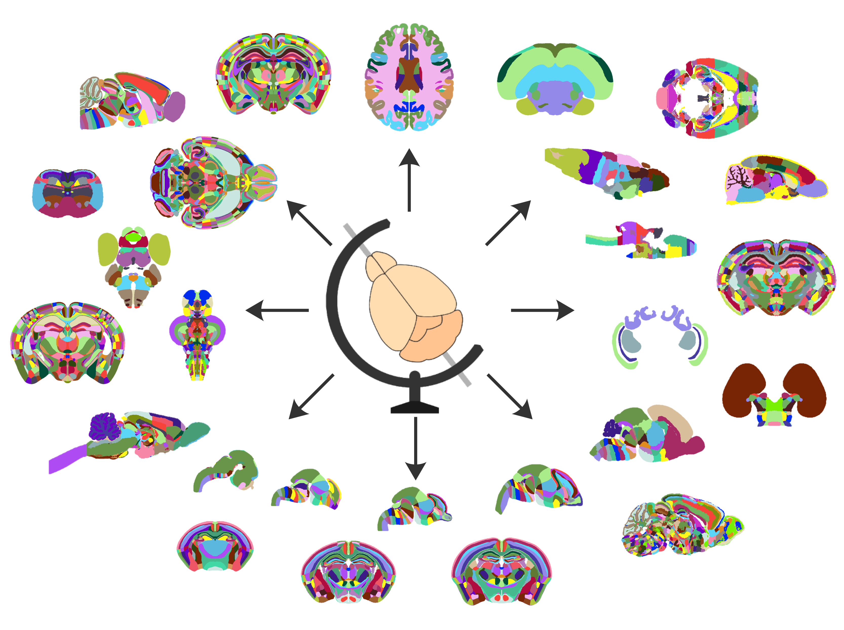
Work with multiple species and atlases.
Collaborate with each other.
neurotwitter, I'm thinking of extending brainrender (https://t.co/ISYhPD7EhE) to atlases other than the Allen brain atlas. Does anyone know where I can download 3D atlases for the rat, drosophila and zebra fish brains?
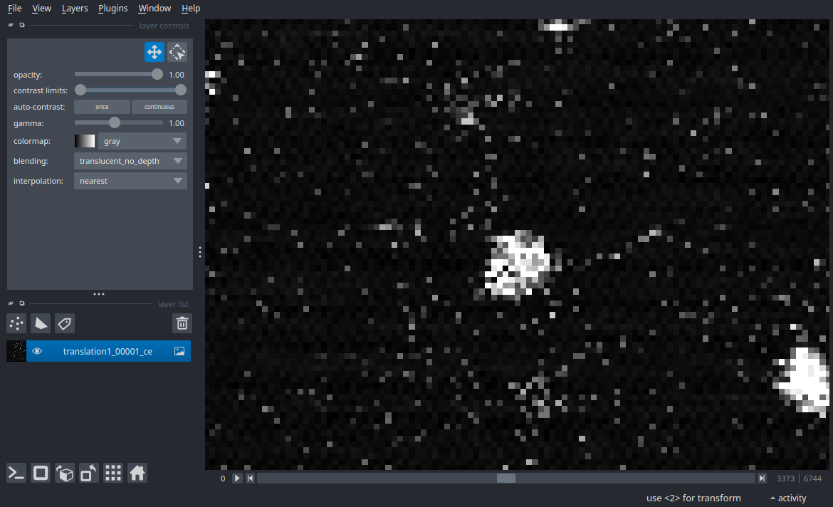
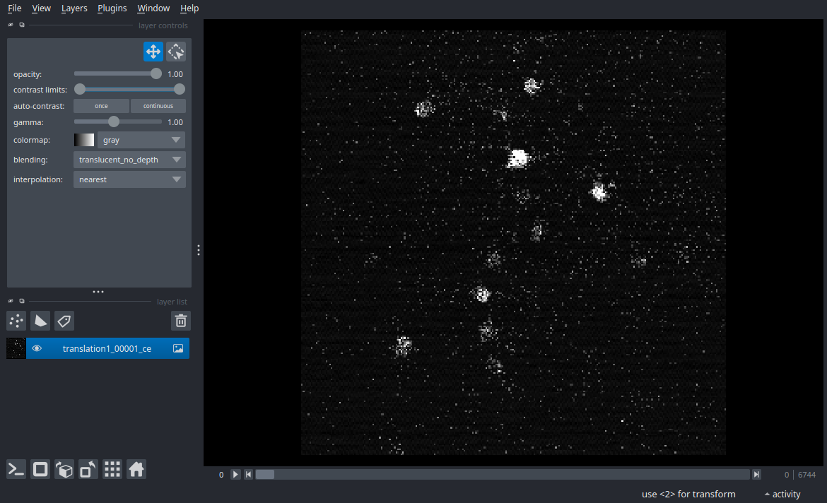
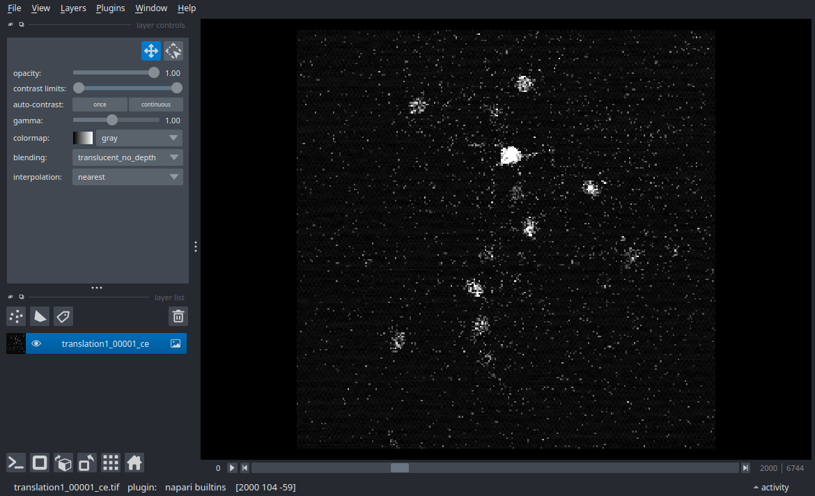
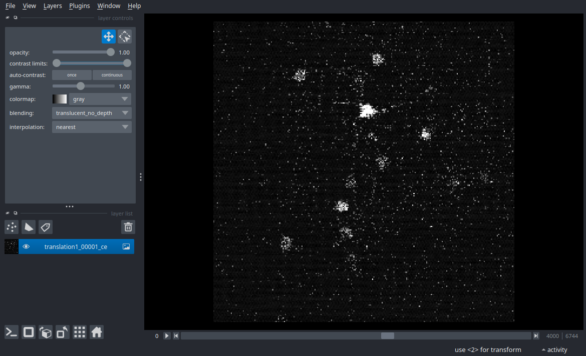
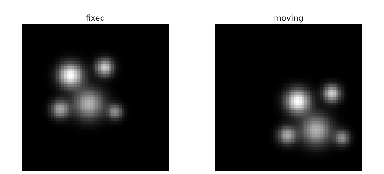
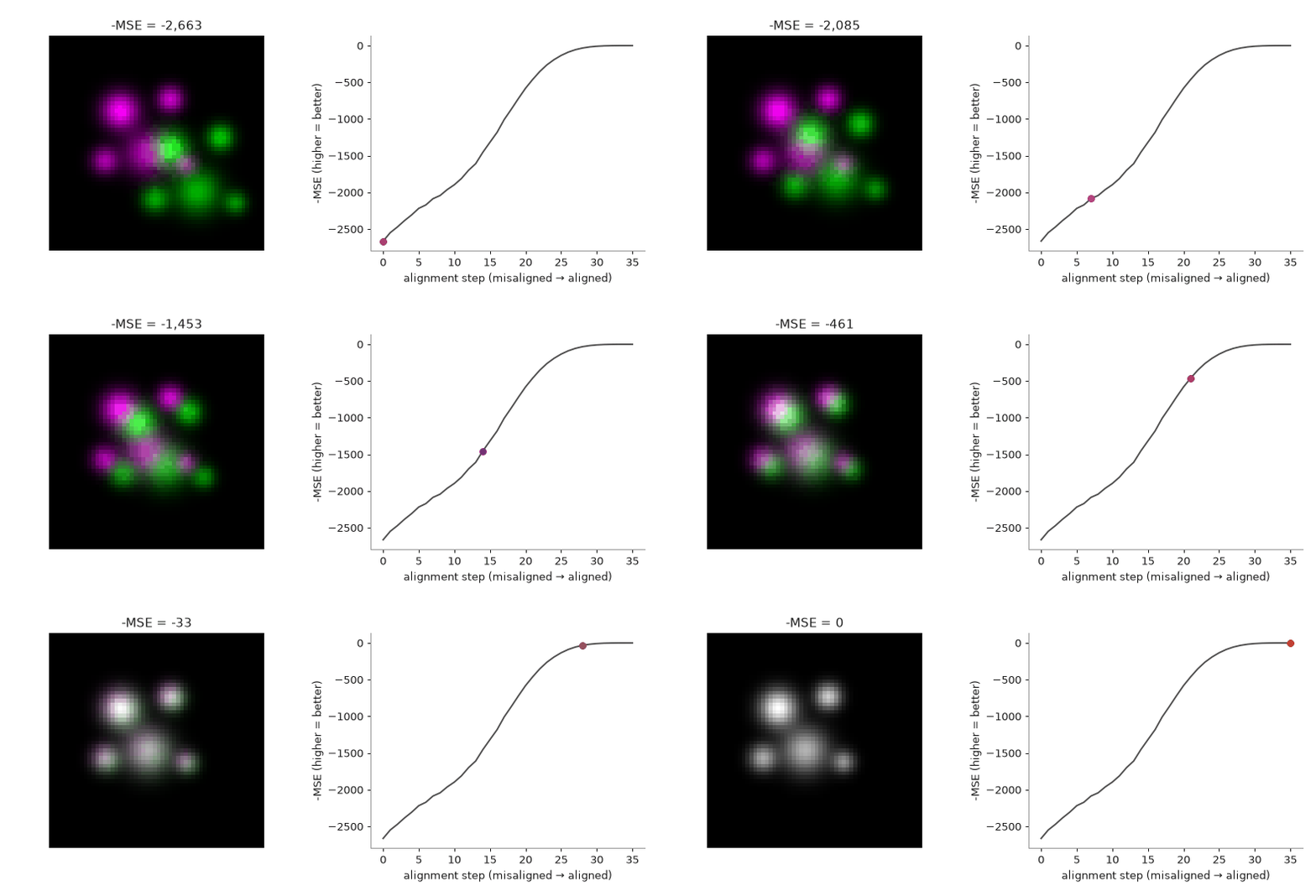
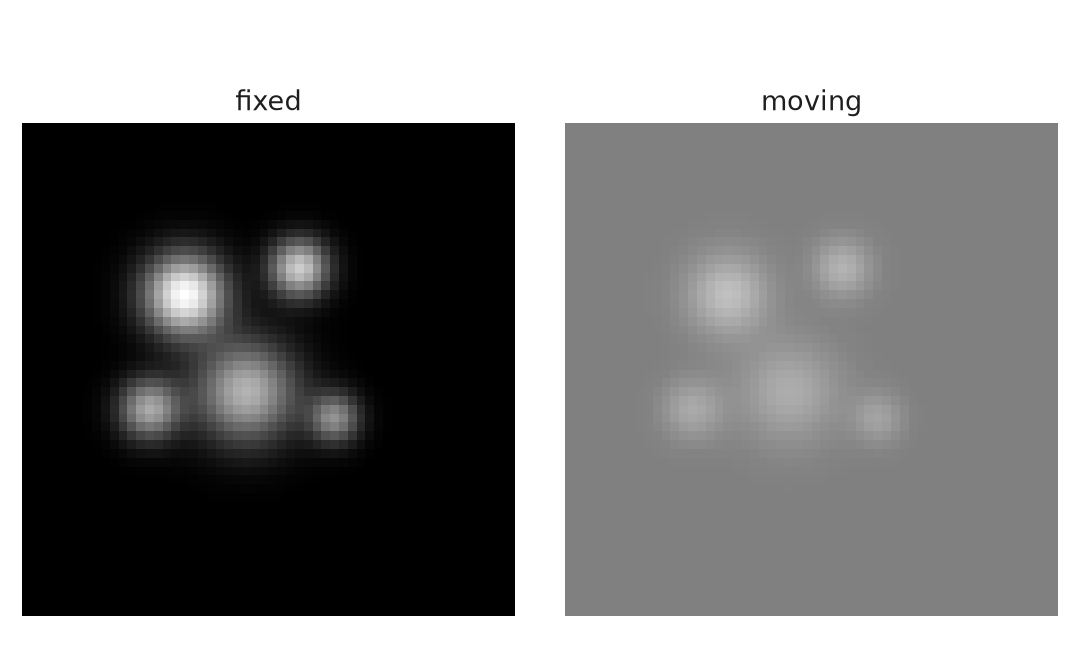
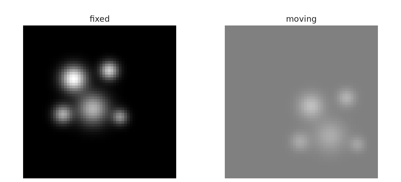
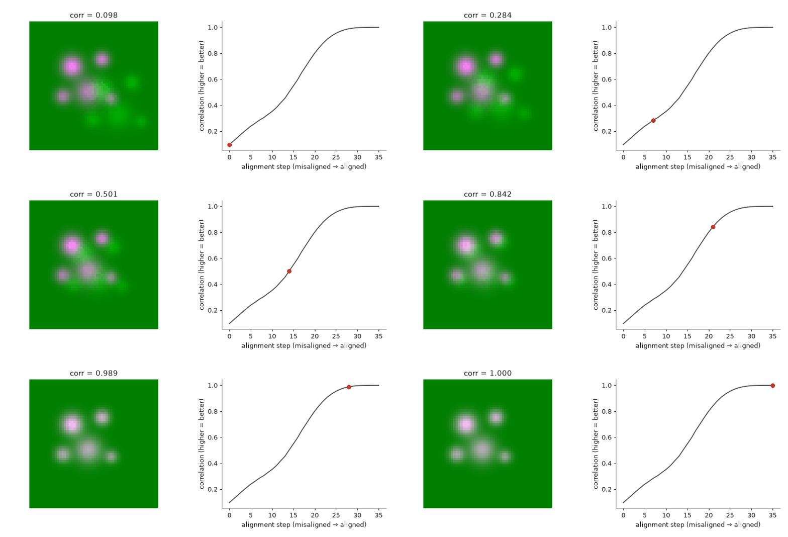
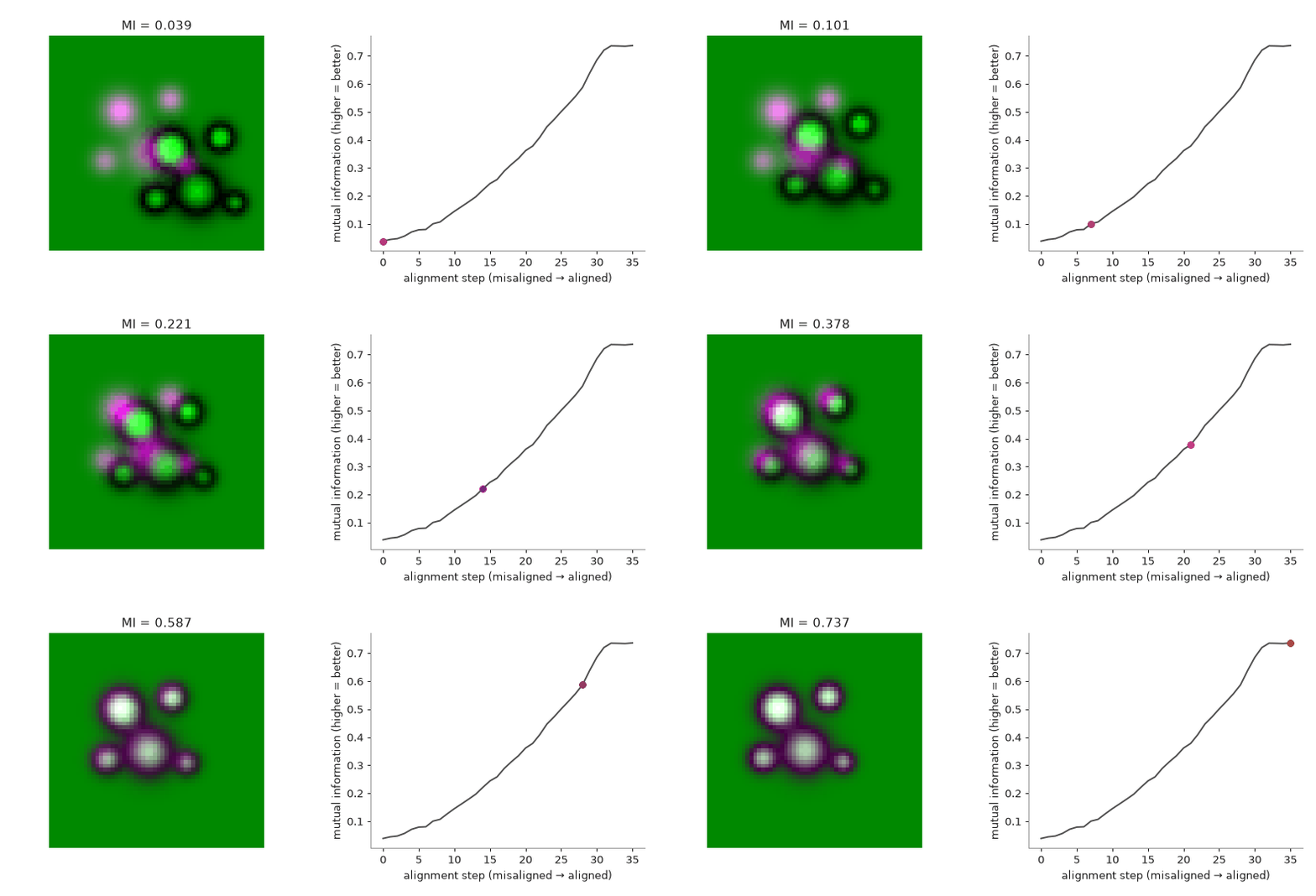
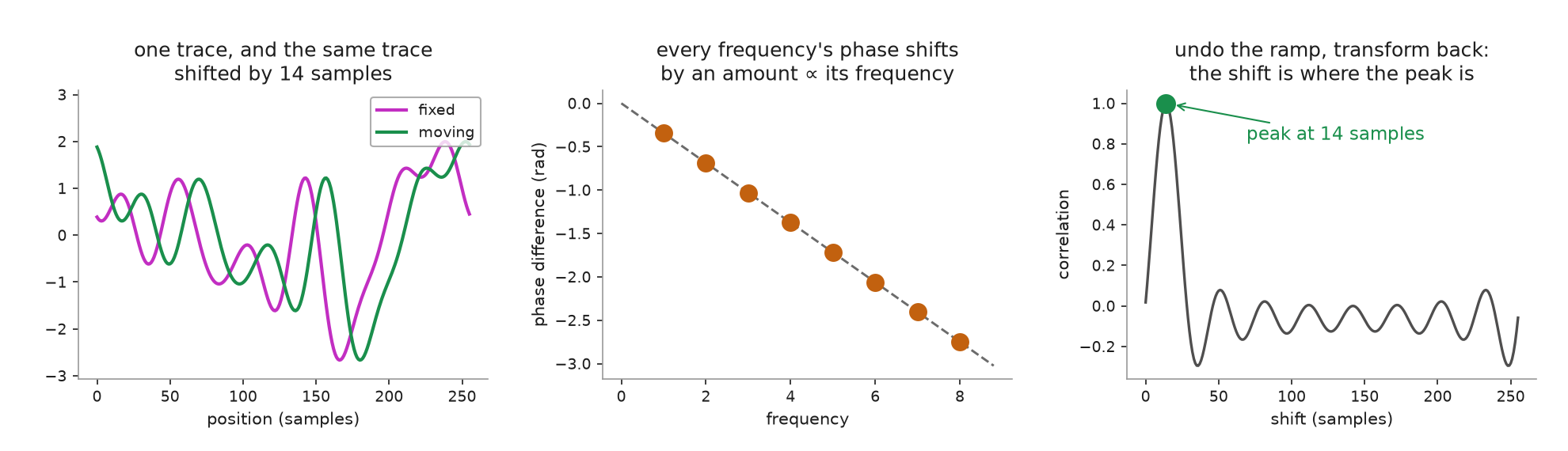
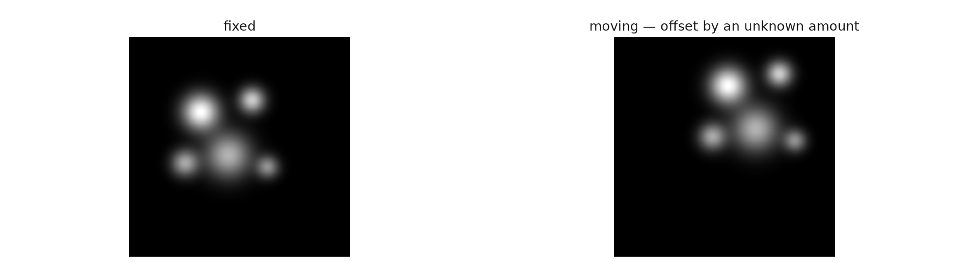
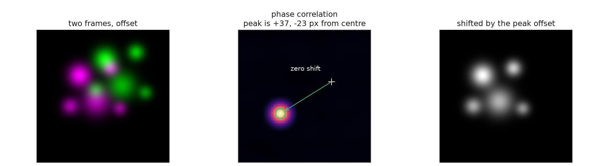
For pure translation, we can compute the correlation between two images for every possible shift at once using the Fast Fourier Transform. Usually called phase correlation.
Phase correlation
Transform both images into frequency space
Combine them with a simple multiplication which gives a normalised correlation in frequency space
Transform back
The location of the peak directly tells you the best-aligning shift
Phase correlation
No starting guess, no iteration, global solution
Fast, and the same cost whatever the shift turns out to be
Only works for pure translation
Rotation, scaling, or warping still needs the iterative route
A good way to get a coarse starting position for that iterative route
Overfitting and Underfitting in Registration
Too much of a good thing
Overfitting and underfitting
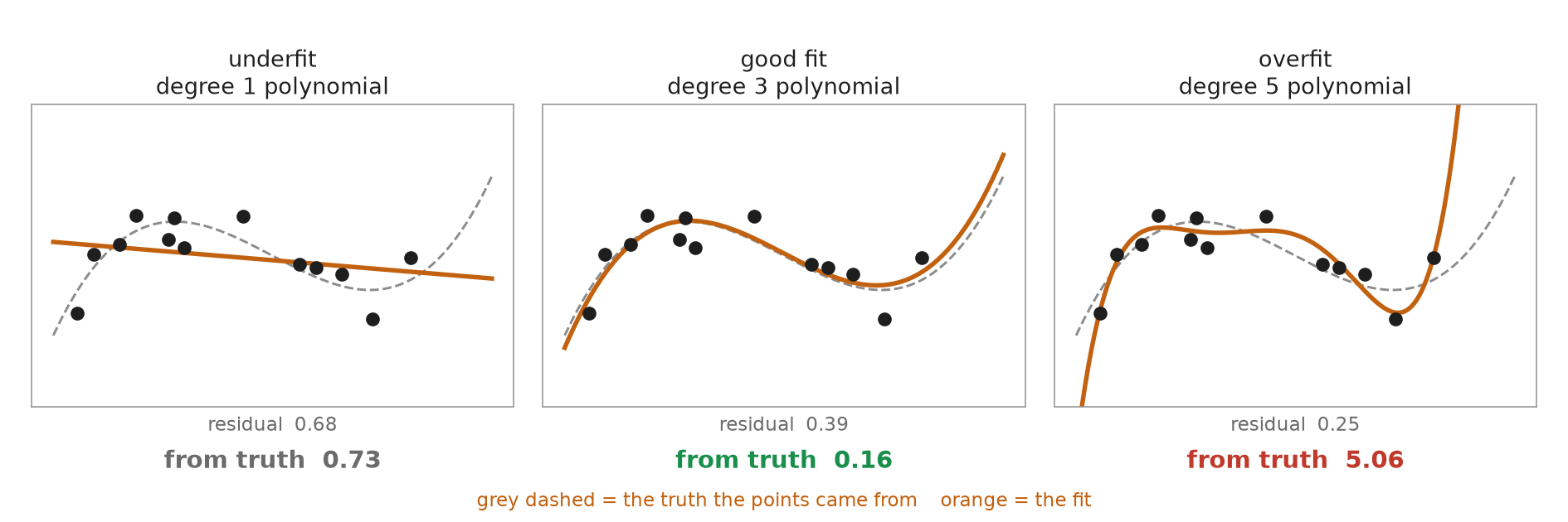
The same trade-off as fitting a curve to noisy measurements
A straight line through curved data misses the real trend: underfitting
A high-order polynomial through every point chases the noise: overfitting
Registration has both failure modes, in two (or three) dimensions
The “model complexity” knob is the transformation type
Underfitting: too many constraints
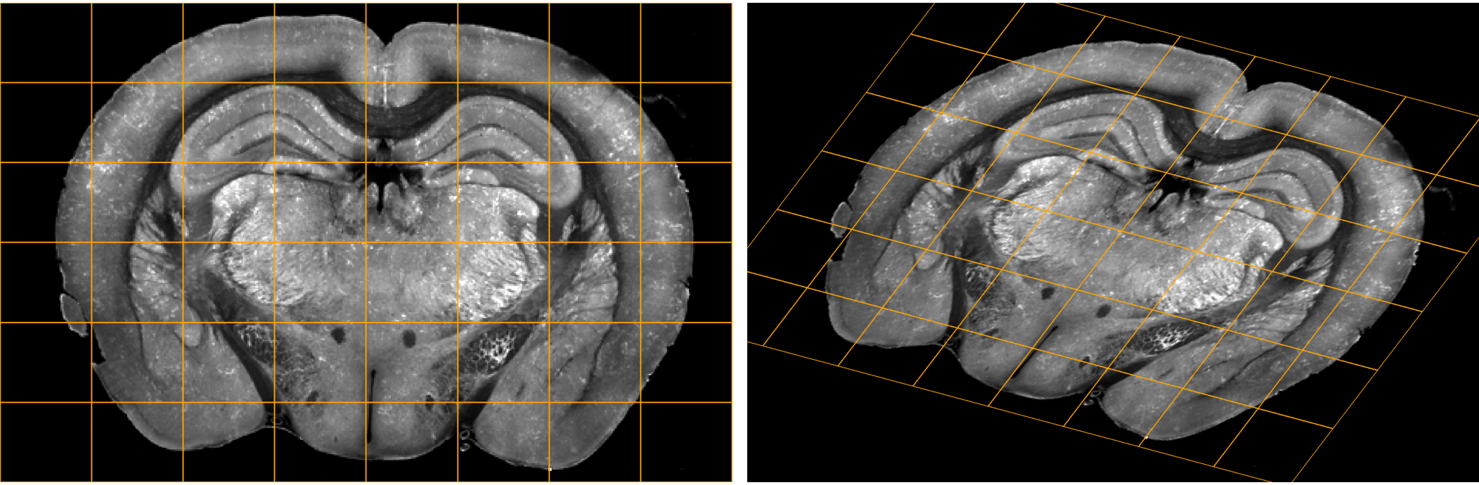
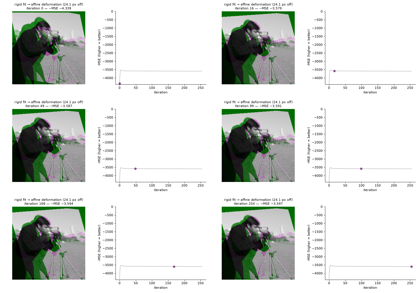
The transformation is too simple to express the real difference between the images
Example: rigid registration of sections that were genuinely stretched and torn unevenly during processing
Symptom: structured misalignment in part of the image, and optimising harder doesn’t help — the transform cannot express the deformation you need
Underfitting: too many constraints
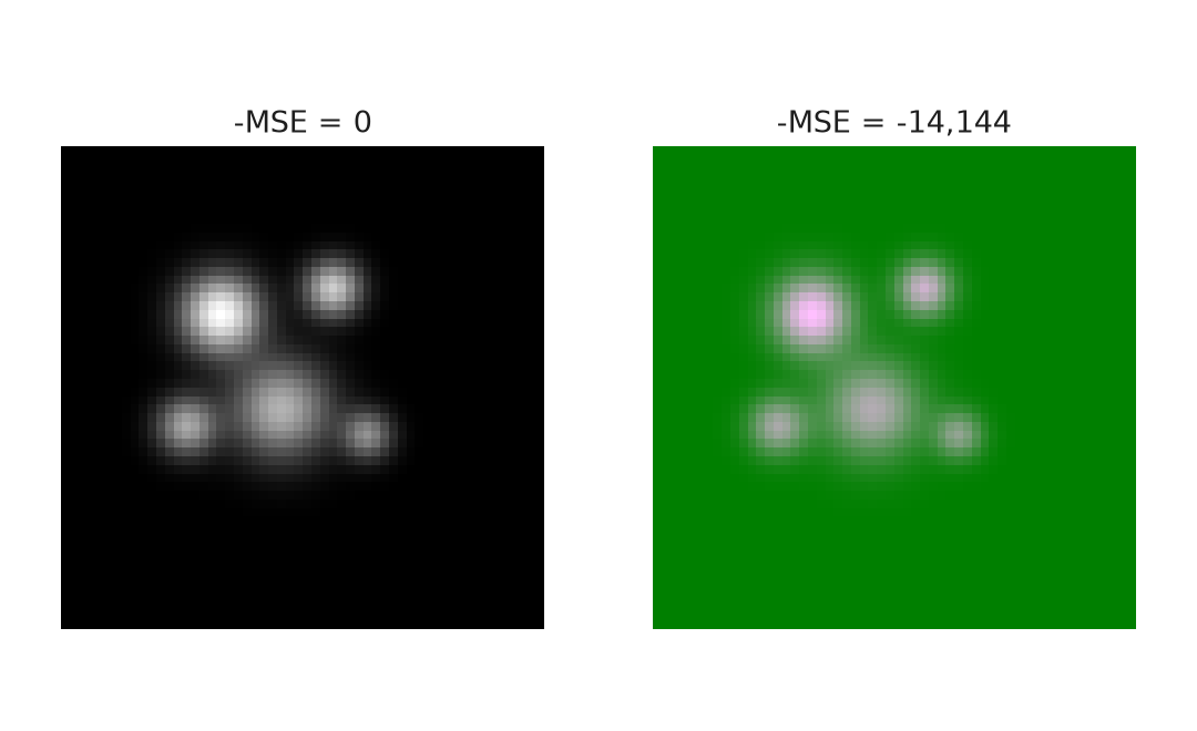
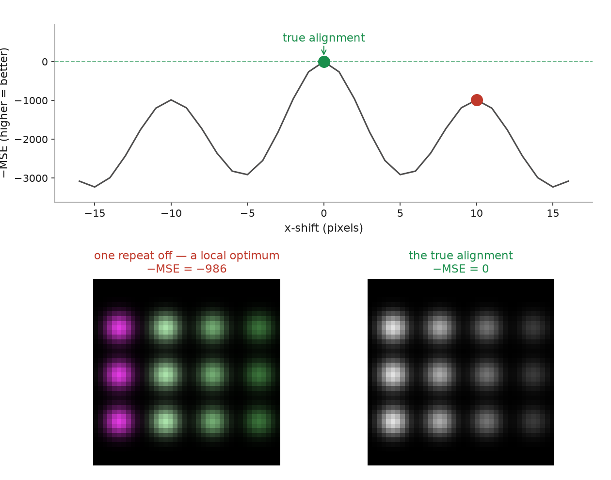
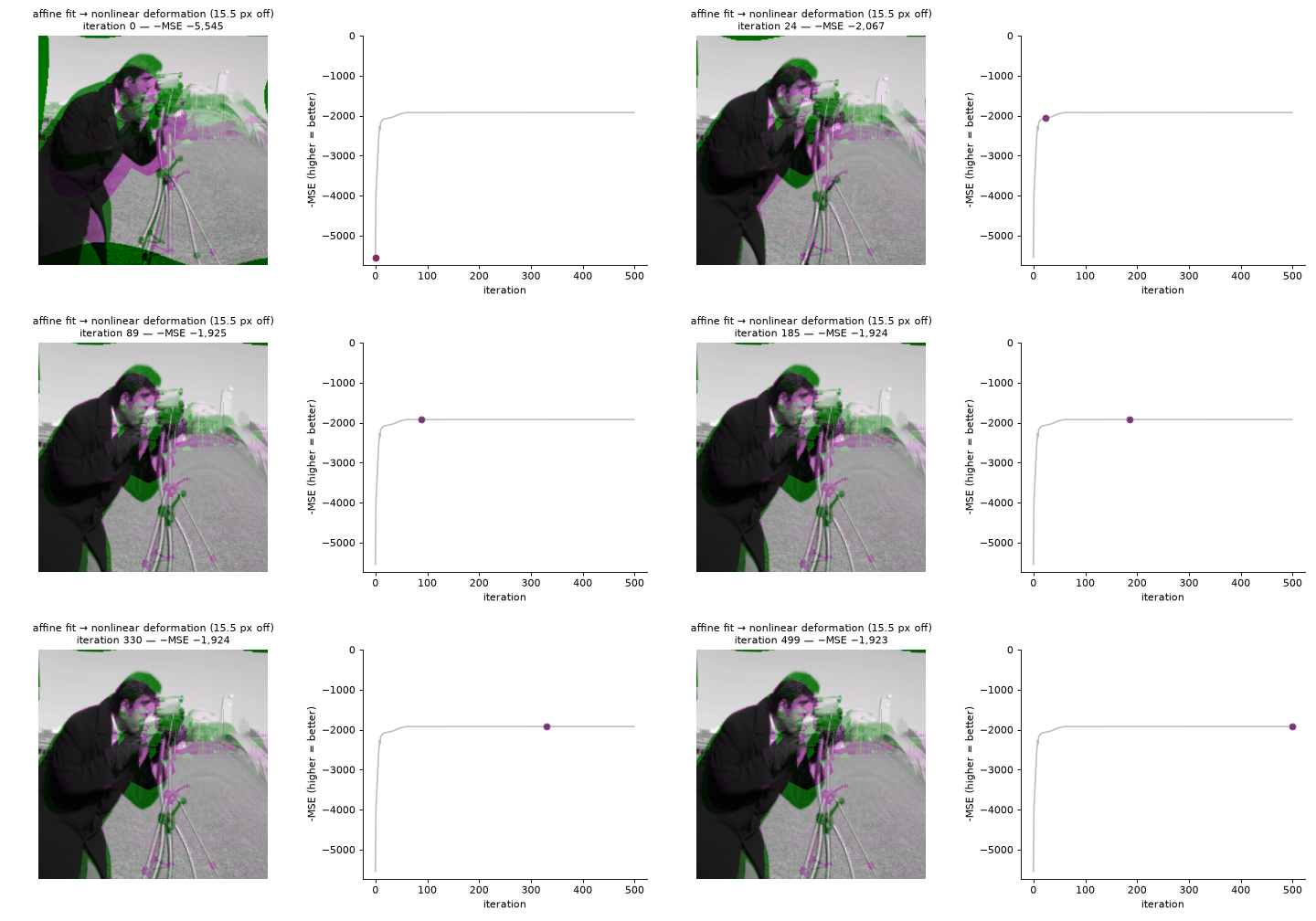
A non-linear warp, fitted with an affine transform — the global stretch comes out, the local warping cannot, and the score flattens out well below zero.
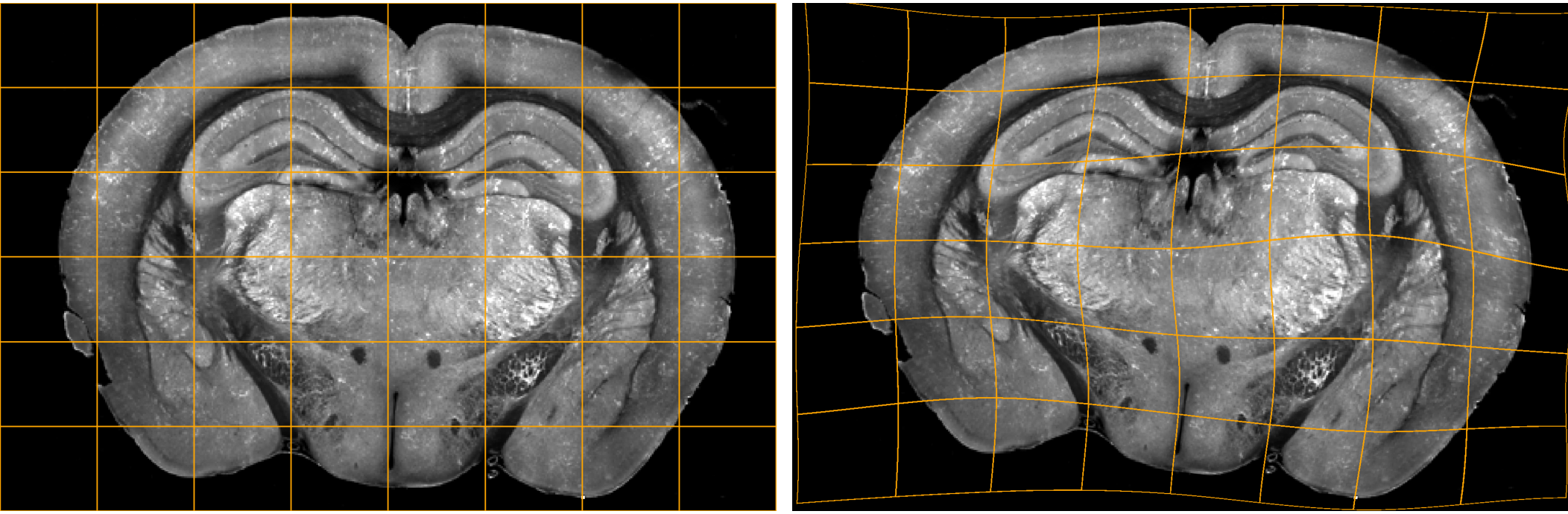
Overfitting: too few constraints
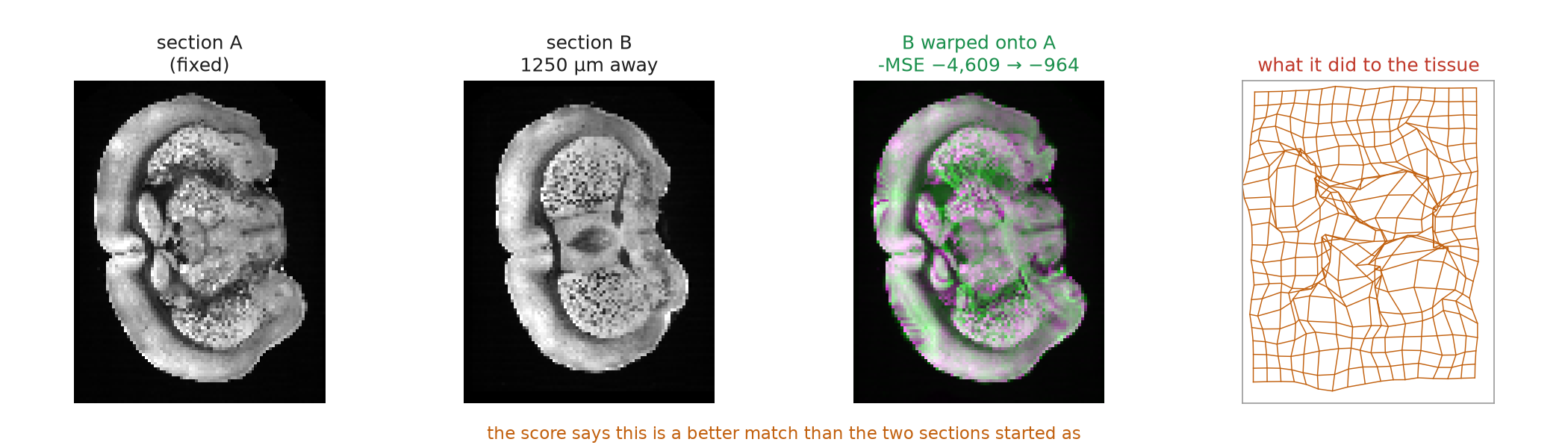
So many degrees of freedom that any two images can be forced to match
A dense B-spline grid with more control points than the texture can constrain
The score looks excellent, but the tissue is folded, implausibly stretched, or matched to structures that shouldn’t correspond at all
Overfitting: too few constraints
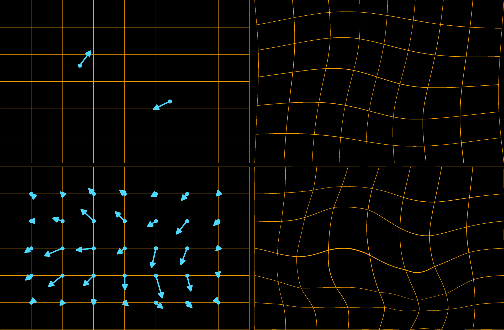
Finding the right level
The right amount of flexibility depends on how much true deformation you expect, and how much data — landmarks, texture — you have to constrain it.
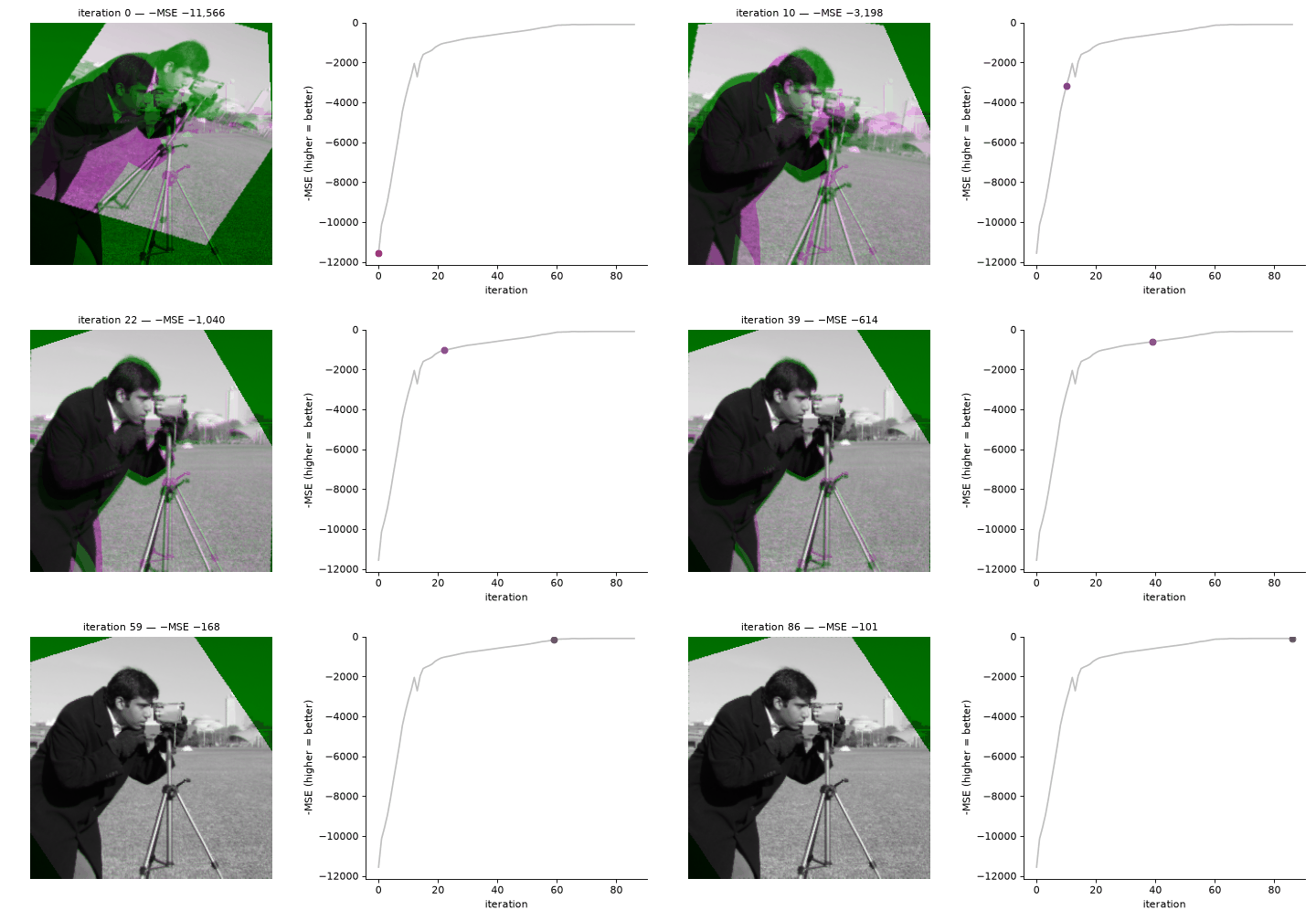
Start coarse and refine — rigid -> affine -> non-linear
Adjust the regularisation terms
Each non-linear method has a way to penalise implausible warps
Use a pyramid / multi-resolution approach
brainreg
brainreg
Pixel-based — no landmarks to pick
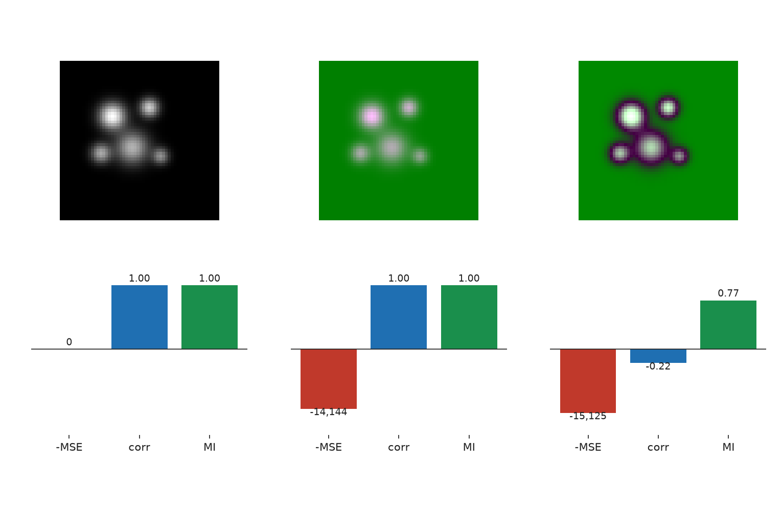
Mutual information — sample and atlas are different modalities
Affine first, then non-linear (B-spline) — coarse to fine
Solves on downsampled data, then applies the result to the full-resolution channels
brainreg: the essentials
Atlas — the target atlas
Data orientation — e.g. psl, the position of pixel (0, 0, 0)
Brain geometry — a whole brain, or a single hemisphere
Voxel size — in microns, one per axis, in the same order as the data
Additional channels have no field of their own — open them as extra layers in napari and they are carried through the same transformation.
brainreg: advanced
Affine / freeform downsampling steps calculate — how many levels the coarse-to-fine pyramid builds
and … steps use — how many of those levels it actually registers on
Grid spacing — B-spline control point spacing; tighter grid, more local flexibility, more overfitting risk
Bending energy weight — the regularisation term; how hard implausible warps are penalised
Smoothing sigma image / atlas — blur before matching, so the optimiser sees shape rather than speckle
Histogram bins image / atlas — how finely mutual information bins intensities before scoring
The defaults are tuned for whole mouse brains
brainreg: tips
Get the orientation and voxel spacing right first
Registration accuracy is the limiting factor, not the resolution of the atlas (typically!)
25 um is usually sufficient for whole-brain registration
Always inspect the result, don’t just trust that it finished
Check the atlas boundaries against real anatomy
Focus on your region of interest
Questions?
Tutorials
Tutorials
Registering whole-brain microscopy to an atlas
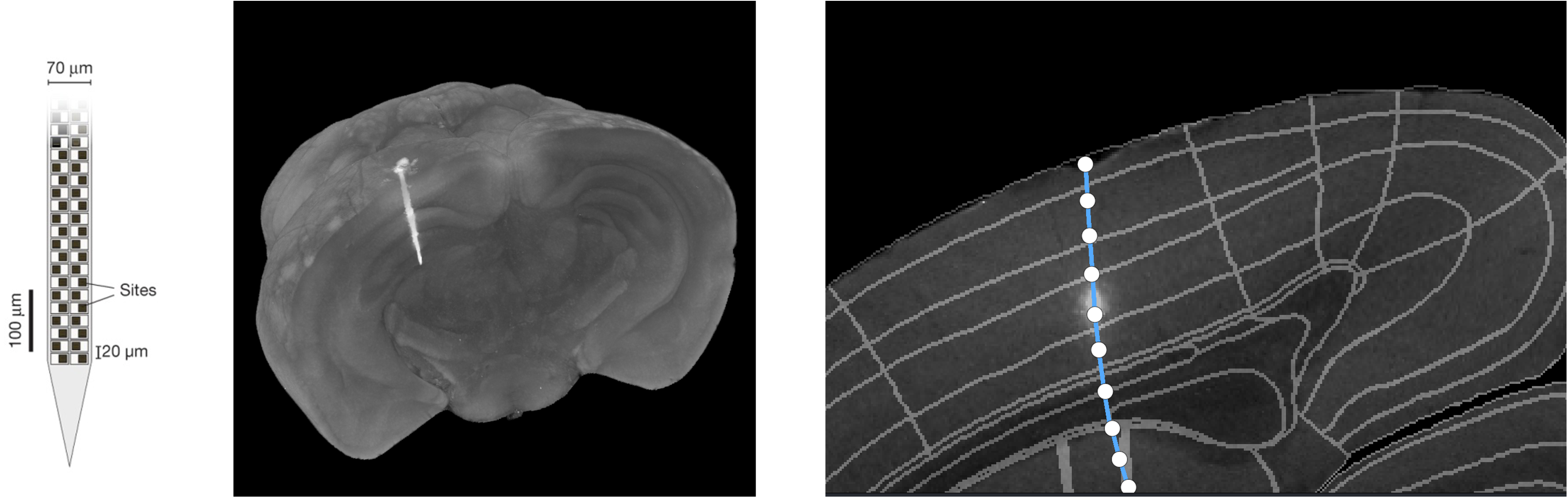
Segmenting probes and bulk fluorescence
Cell detection in whole-brain microscopy
Retraining cellfinder to fine-tune cell detection
Combining registration and cell detection
Scripting with BrainGlobe
Data
Small sample data comes with napari
Large sample data brainglobe-course-data/MS_cx_left
on HD: share if needed
Quick excursion into BrainGlobe orientation
three letters define position of pixel (0,0,0)
e.g. psl - pixel (0,0,0) is Posterior, Superior, Left
all BrainGlobe atlases are asr
to verify: open data in napari and scroll through data
demo
Registering whole brain microscopy images with brainreg
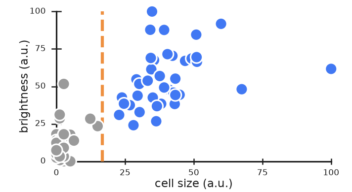
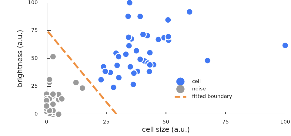
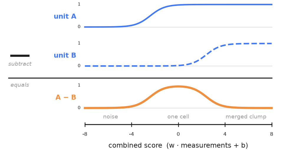
3 px wide, brightness 109 → score −4.5 → not a cell
Real data is complex!
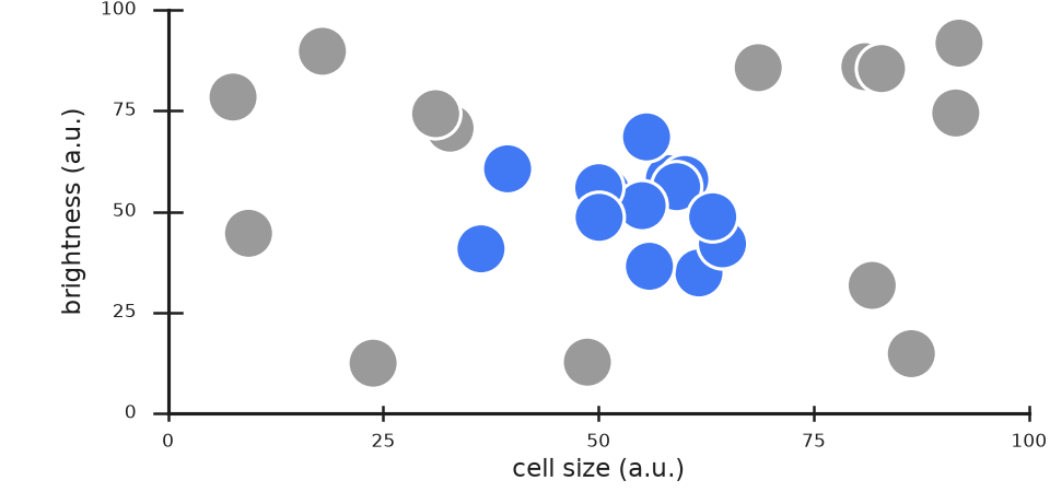
No straight boundary can separate these two groups - wherever you put it, it cuts through the wrong points
Fitting complex relationships
Change the question from “is this a cell?” to “is this exactly one cell?”
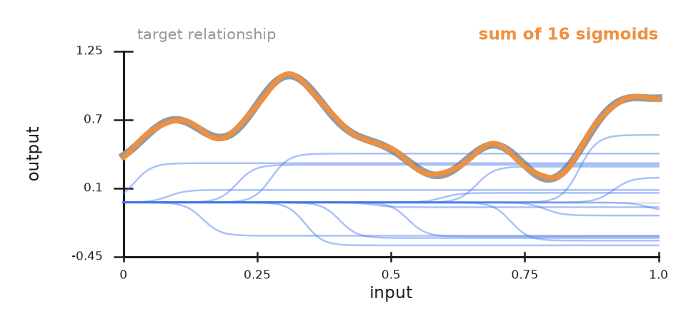
Fitting complex relationships
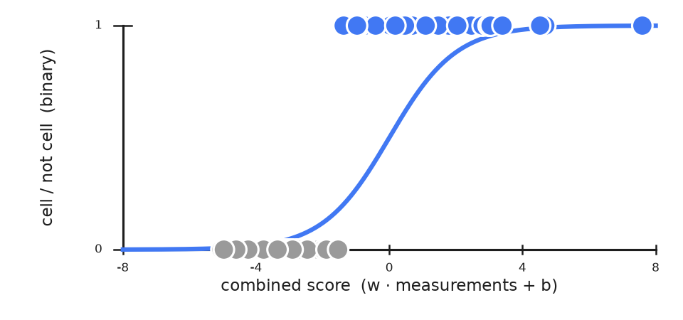
Nothing about the target is sigmoid shaped. Add enough single sigmoids, each with its own fitted weight, and the sum can take essentially any shape.
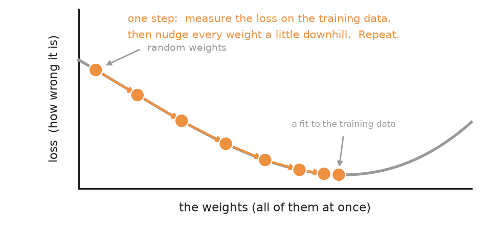
How the weights are found
Relies on having a loss that estimates model performance
What is a neural net?
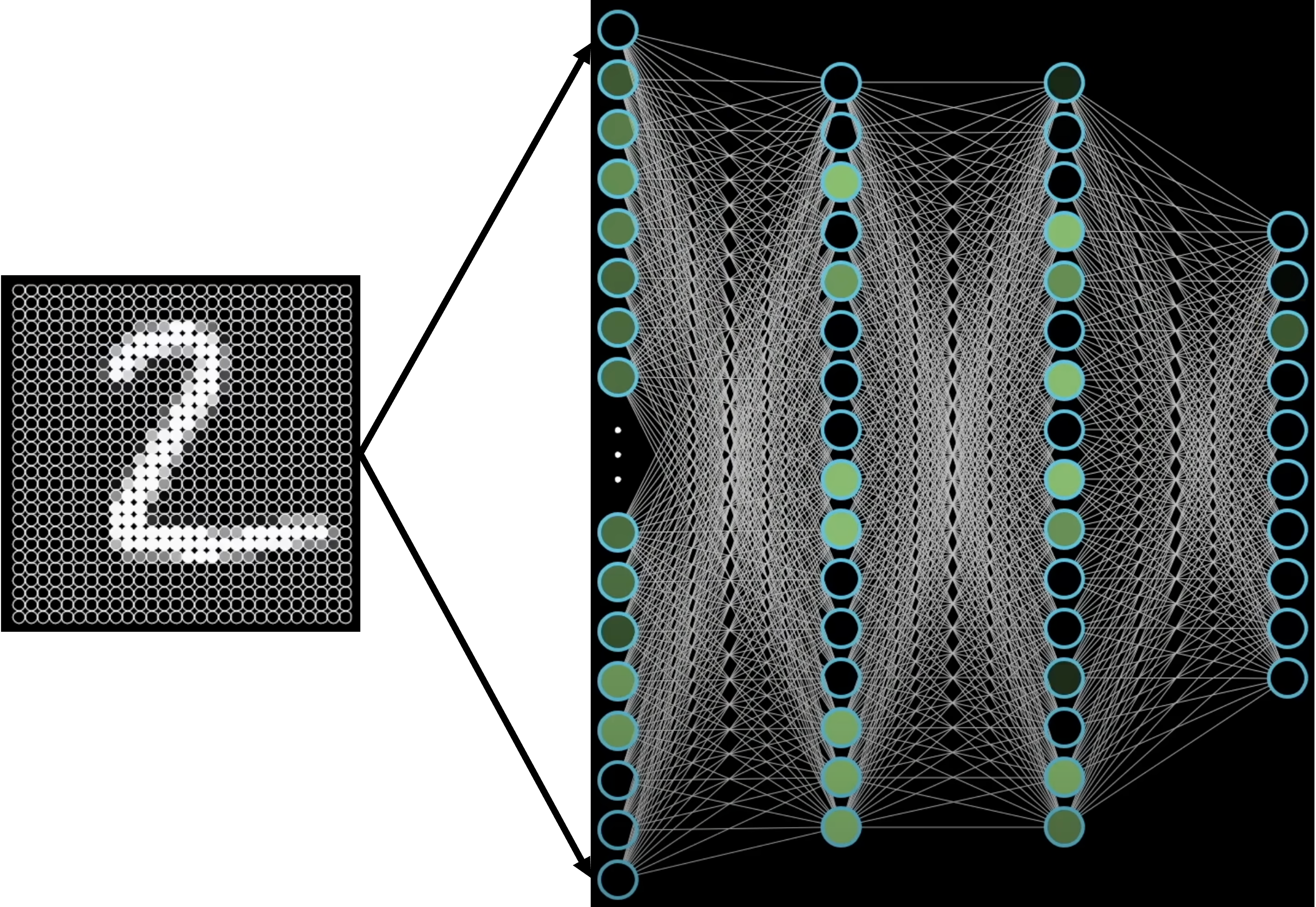
A combination of units
Every pixel feeds every unit in the first layer, and each unit is the same as the last few slides: a weight per input, a bias, a squash. The ten outputs are: [0, 1, 2, …, 10]
Architecture: wiring the units
Fully connected layers: every unit in one layer connects to every unit in the next
Convolutional layers: each unit only connects to a small patch of the previous layer
Transformer layers: every unit can read every other, but how much it reads each one is computed from the input itself
All of these are just different ways to wire up regression units.
Building your training set
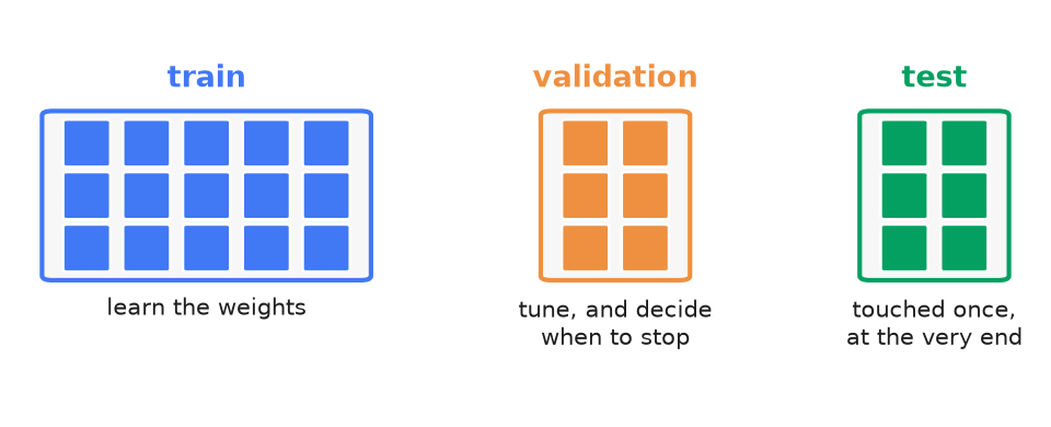
Train, validation, test split
Split the data once, three ways — and treat the test set as spent the moment you look at it.
Memorising practice answers != learning biology.
Test set leakage
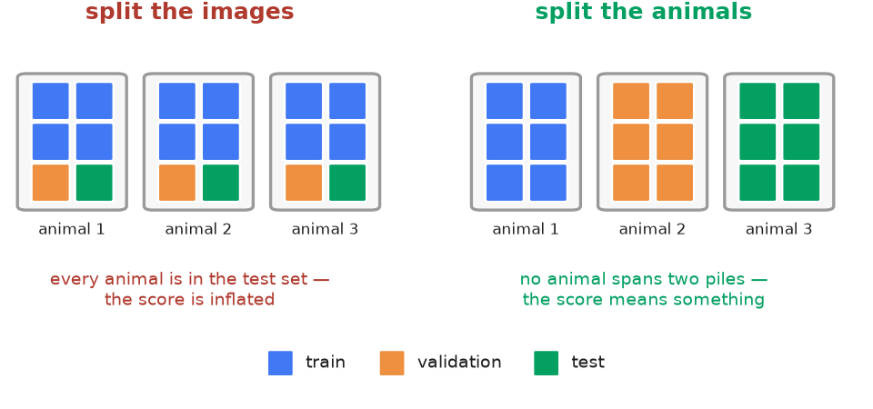
Splitting images randomly isn’t the same as splitting subjects randomly
If one animal contributes images to both the training set and the test set, the model can partly identify it: same tissue, same staining batch, same imaging session
The test score then reflects memorisation of that subject, not real generalisation
Fix: split by subject (or by acquisition session) first, then assign every image from that subject to train, validation, or test — never split across
Split the animals, not the images
Statistical not causal
A model learns whatever correlates with the label, which may not necessarily be the biology!
Chest X-ray models trained to detect COVID-19 were found to rely on features outside the lungs entirely — image borders, laterality markers, patient positioning
If every positive scan came from one hospital, the model can learn that hospital’s scanner artefacts instead of the disease
The model is statistical, not causal. It will happily use a confound if the confound is easier to learn than the real biology.
Scoring a model
Every claim about performance is one number, computed by comparing predictions to labels on one split
Accuracy — fraction of calls that were right. Misleading when one class is rare: call everything “background” in a sparse image and you score 99%
Precision — of the things you called cells, how many were cells? Low precision = false positives
Recall — of the cells that were there, how many did you find? Low recall = false negatives
F1 — a combined metric, so a model can’t win by being timid or trigger-happy
Precision and recall trade off: lower the detection threshold and recall goes up while precision goes down
Generalisation
A model that generalises scores as well on unseen data as on training data
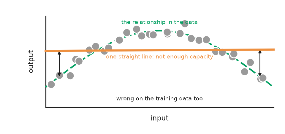
Underfitting: too little capacity, or too little training — poor on both
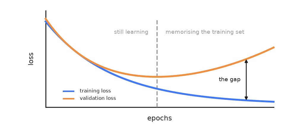
Overfitting: enough capacity to memorise the training set — good on train, poor on test
Test labels are human opinions too. 95% recall against one annotator’s boundaries is not 95% against the biology.
Underfitting
Too little capacity to represent the relationship at all - so it is wrong on the training data as well as on unseen data
Overfitting
Too much capacity, the model memorises the training data without extracting any information
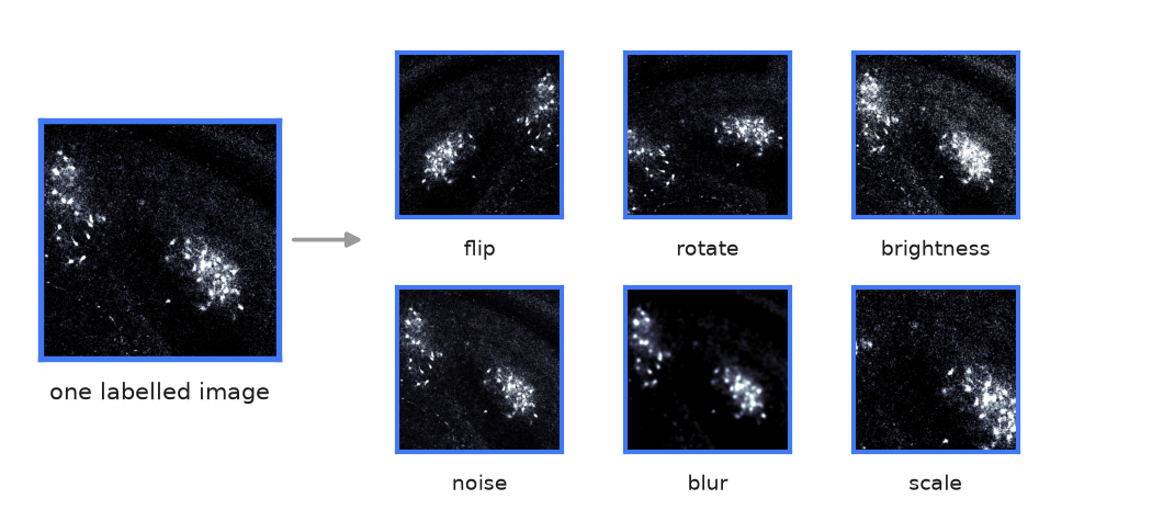
Data augmentation
Labelling is the expensive step: make more training examples out of the ones you already have!
Flip, rotate, rescale, brighten, blur, add noise
The model sees a sample at more orientations, brightnesses and noise levels
Microscopy has no up, so flips and rotations are free
Data augmentation
Augment the training set only
Split first, augment second — a flipped copy of a training image landing in the test set is the leakage problem again
Validation and test sets stay untouched: they have to look like the data you’ll actually face
Augmentation buys invariance, not new biology. 500 copies of 10 animals is still 10 animals!
From pixels to meaning
Pixels don’t scale
784 pixels for a thumbnail digit — a single tile of imaging data is millions. Almost all of it is empty background! The actual information is sparse
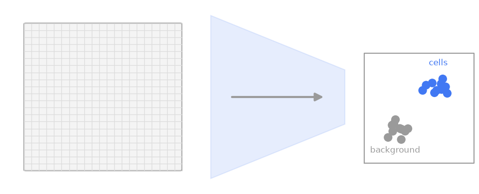
The compression funnel
pixel space
millions of numbers, mostly redundant
embedding space
a few hundred numbers, in which like sits near like
Convolutional Neural Networks
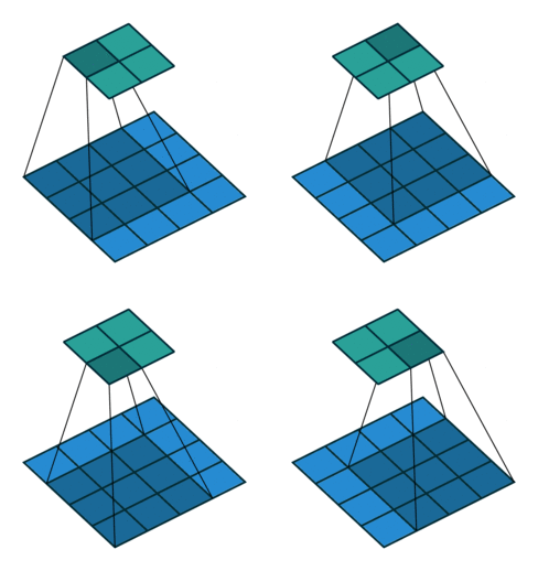
A window that slides
The same small window of weights is applied everywhere in the image
Where it matches, it writes a high value into a feature map
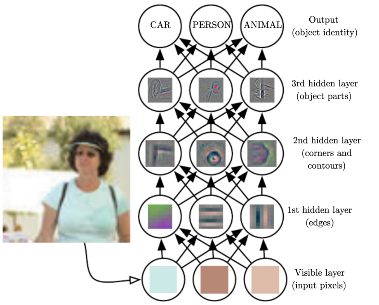
Increasingly abstract spotters
Early layers find edges; later layers combine them into shapes, then parts, then a name
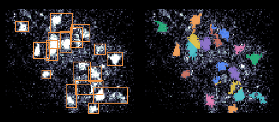
Detection vs segmentation
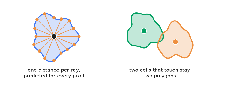
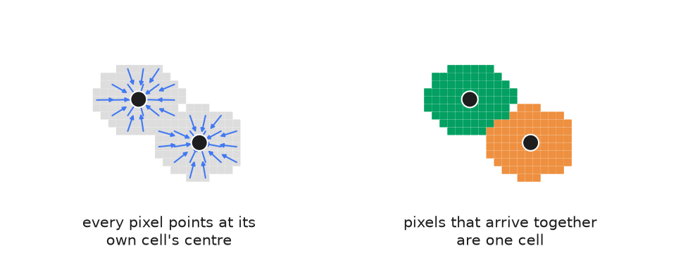
Detection — a point per cell
Segmentation — every pixel is a cell or background
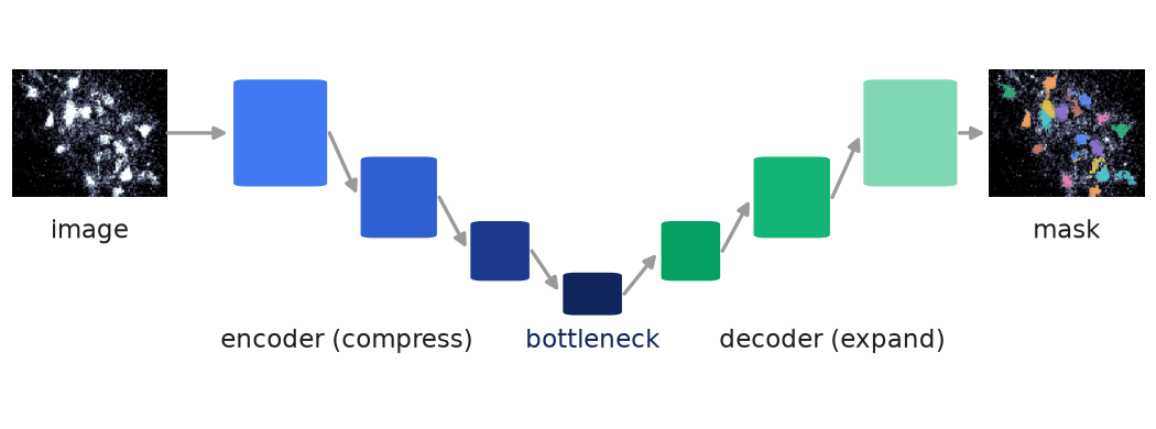
U-Net: built for segmentation
The U shape
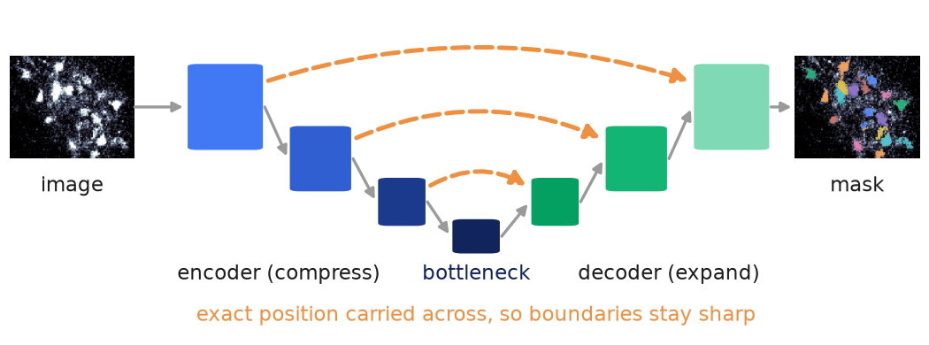
Zoom out for context, zoom back in to trace the exact outline.
Skip connections
Without them the decoder only has the blurry bottleneck to work from.
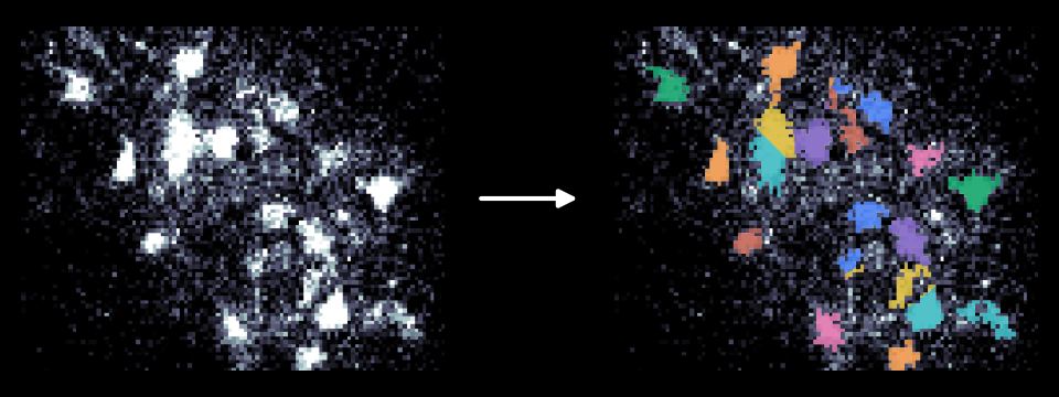
Input -> precise mask
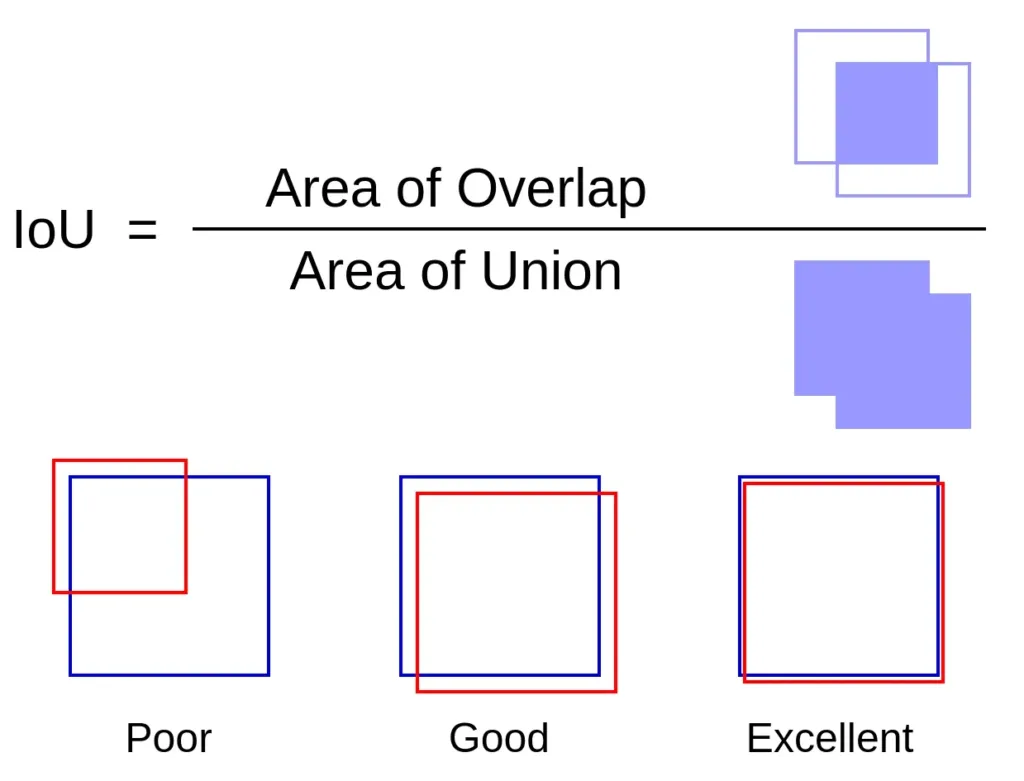
Scoring a mask: IoU
Precision and recall need a rule for when a predicted cell is a labelled cell. For masks, that rule is overlap.
Vision Transformers
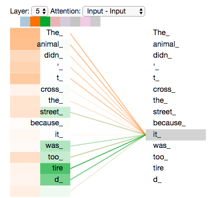
Attention, in words
In “the animal didn’t cross the street because it was too tired”, what does “it” refer to?
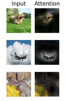
Attention, in images
Same idea on pixels: the model decides for itself which parts of the image matter
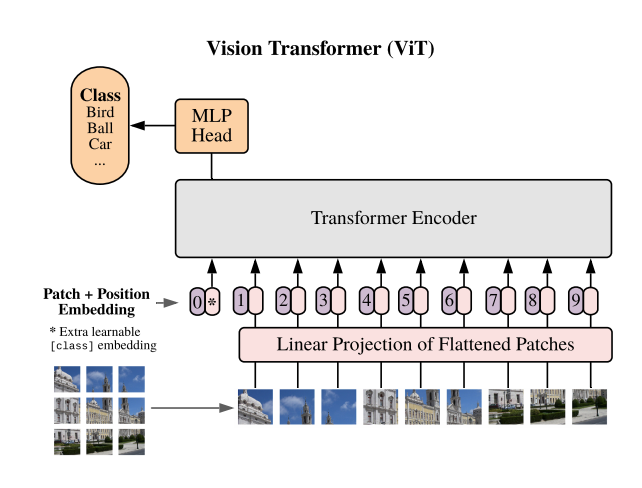
ViT: patches, like words
The image is cut into fixed-size patches, and each patch is treated like a word
The stack of patches goes through the same machinery to generate an embedding
A simple network on top can use this embedding to predict the output
From scratch vs fine-tuning
Training from scratch
Complex model architectures take longer to train and need more data
Large foundational models are trained on 100k - 1 billion images!
cellfinder was trained on 100k hand labelled cells
Generating the data takes too long
Fine-tuning
Starting from random weights doesn’t always make sense!
Sometimes you want to reuse the encoder/embeddings from other models
Feed a small number (100s to 1000s) of your data to teach the model “your” data
Human-in-the-loop
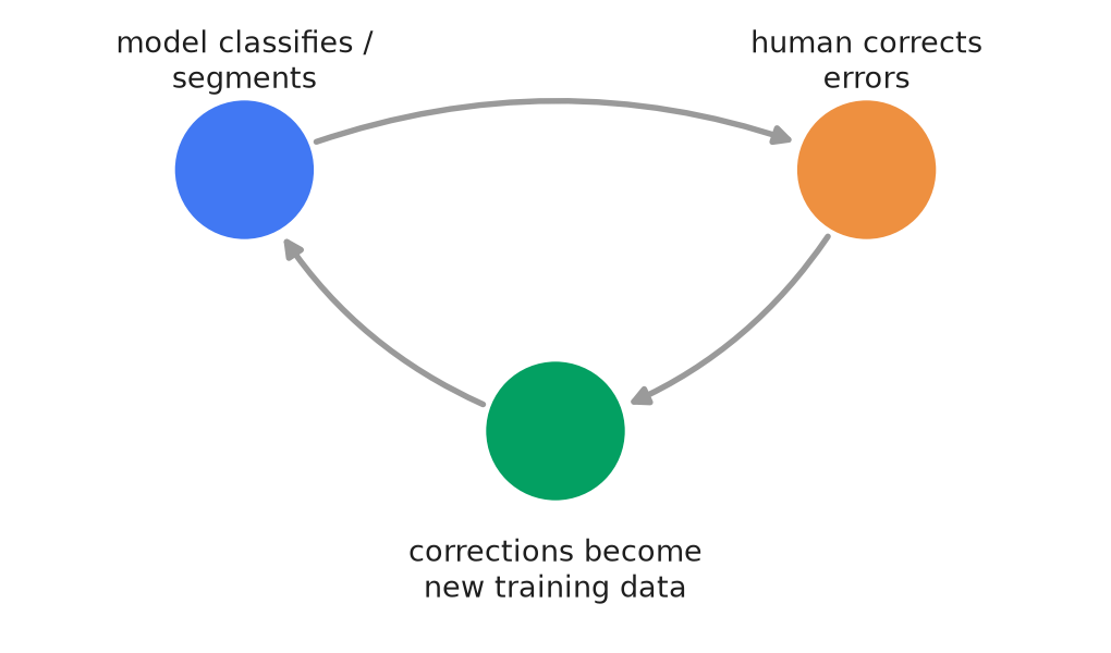
Most fine-tuning data comes from correcting the model’s own mistakes.
ViT backbone, trained on SA-1B: ~11 million natural images, ~1 billion masks — of which only ~10 million over ~300k images were drawn by hand; the rest the model generated and a filter kept
Promptable: click a point or drag a box, get a mask — no retraining
Knows “object”, not “cell”, out of the box it does poorly on microscopy images
Takes SAM’s pretrained ViT backbone and trains it on Cellpose’s cellular datasets
Deliberately trained against realistic degradations — blur, noise, anisotropy, channel order — so it holds up on data it hasn’t seen
Approaches human-to-human agreement on their test set
cellfinder
Detection for large 3D imaging datasets
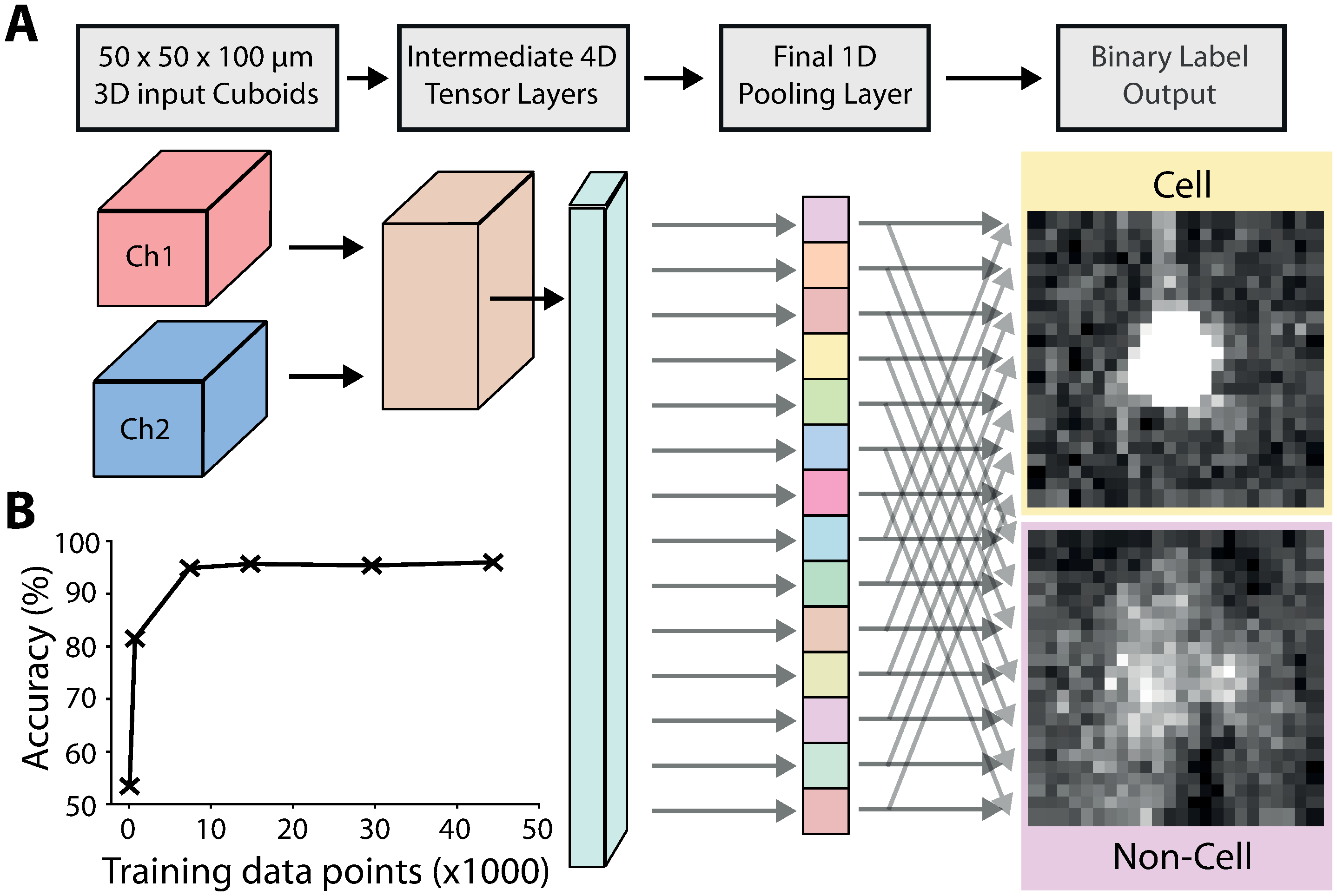
Classical filtering proposes candidate cells; a small CNN classifies each candidate as cell or artefact
Detection, not segmentation: counts and coordinates not outlines
Ships with a pretrained network, which can (should!) be fine-tuned
Tomorrow
Tomorrow you’ll retrain cellfinder on your own corrections — fine-tuning and human-in-the-loop, on real data.
Questions?
Cell detection with cellfinder
3D Cell Detection
cellfinder
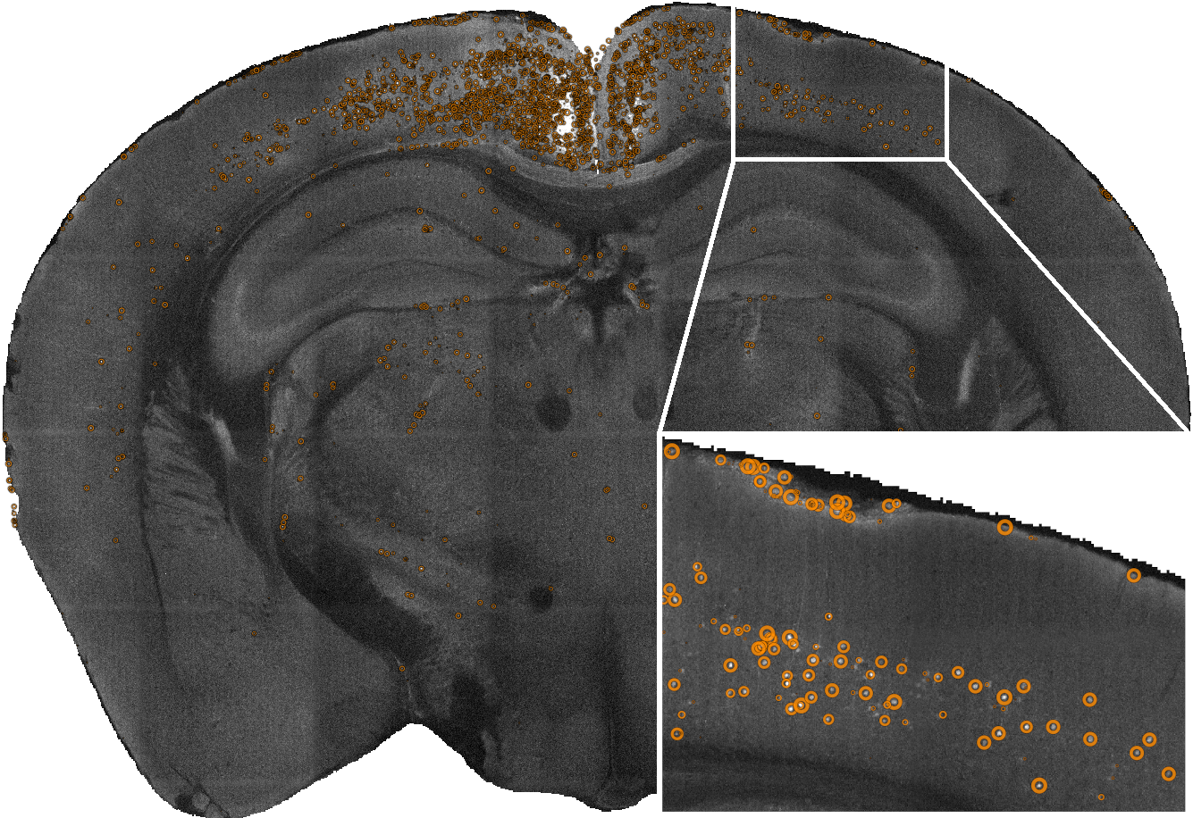
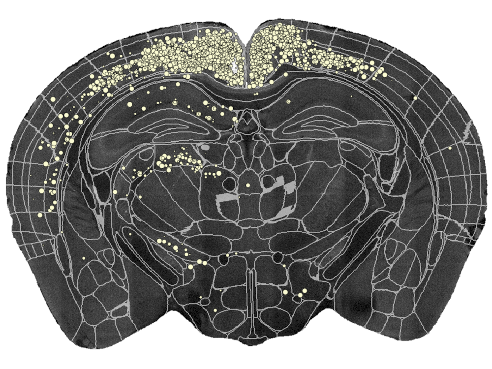
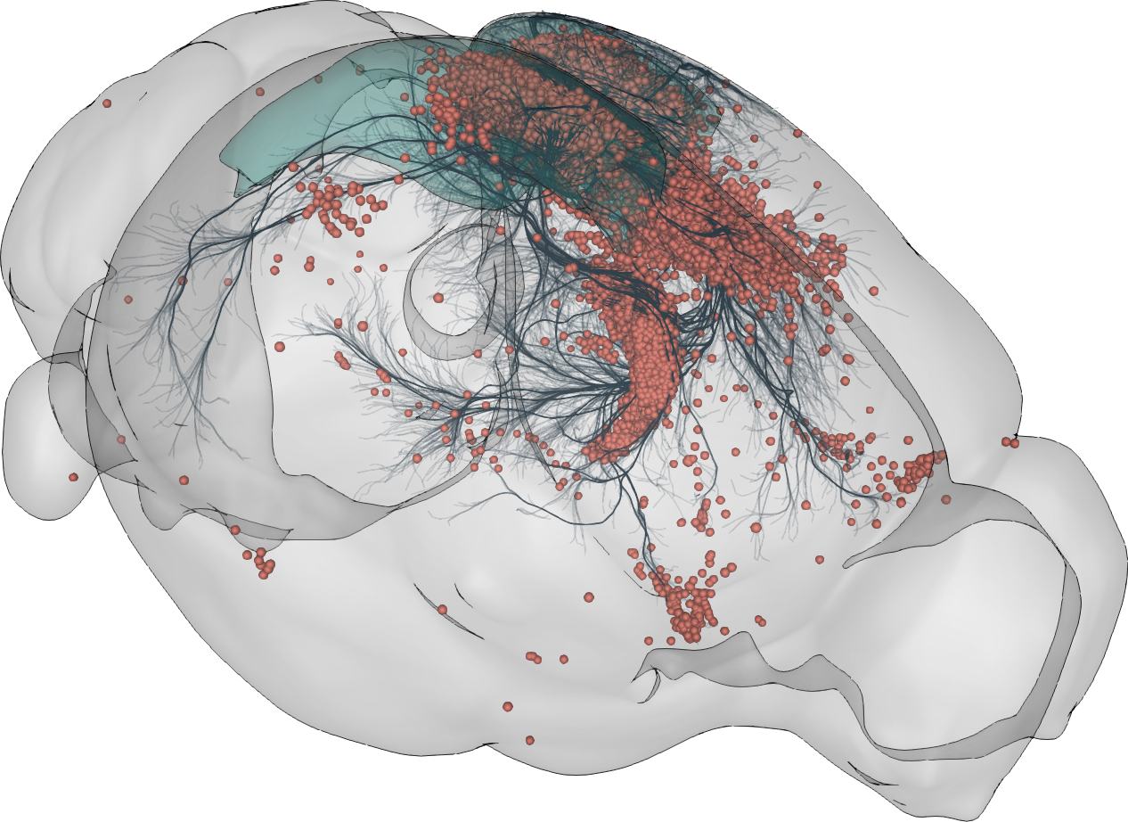
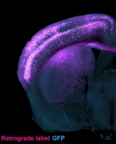
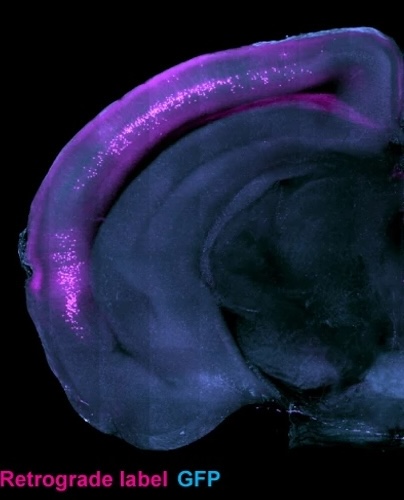
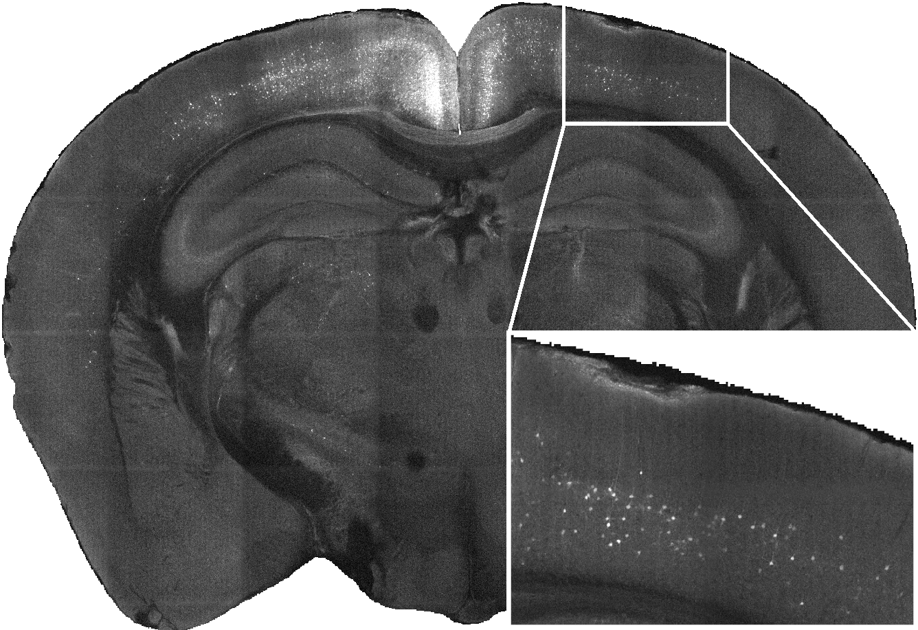
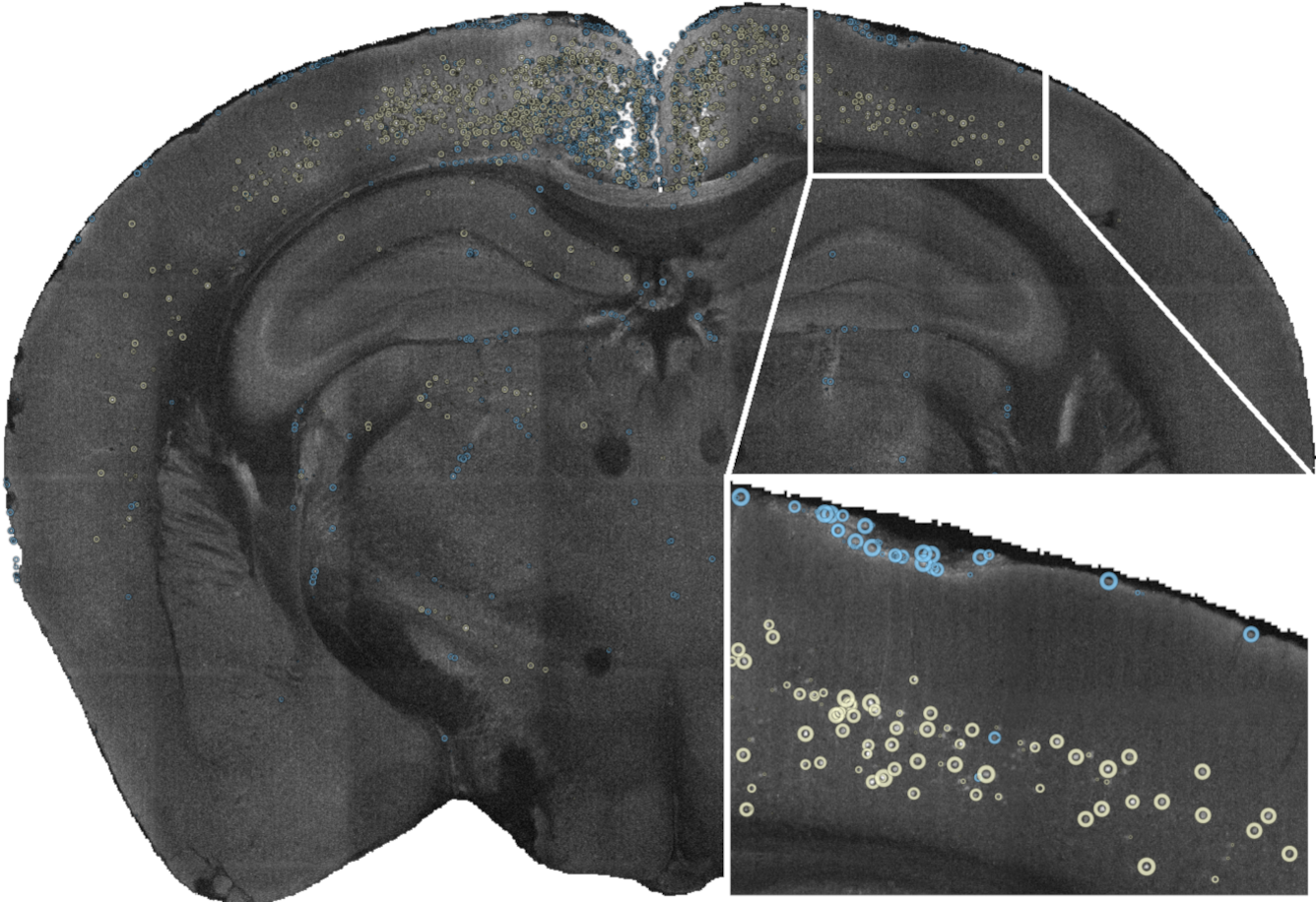
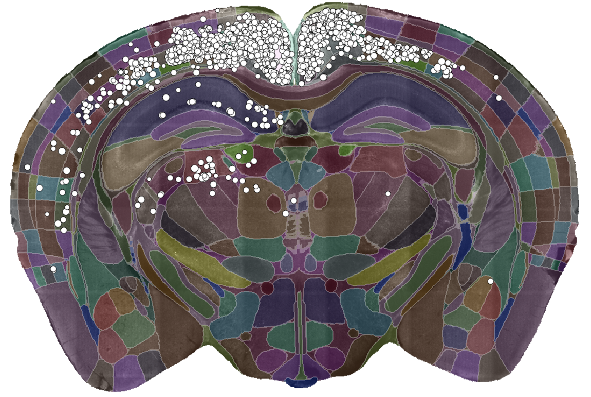
cellfinder is the BrainGlobe tool for detecting cells
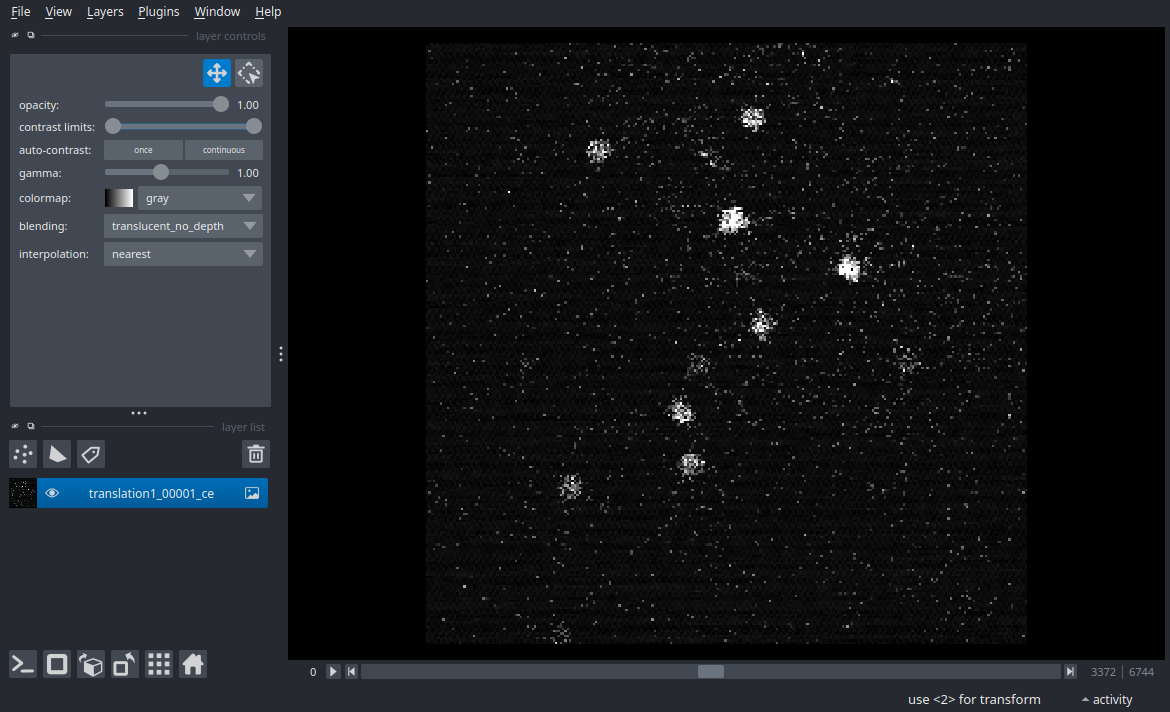
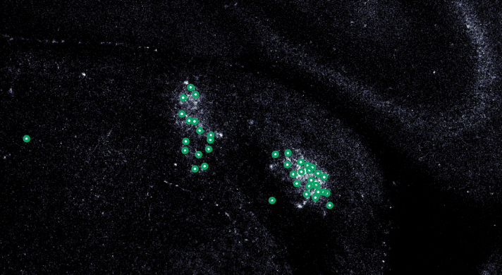
It finds centre coordinates of fluorescently labelled cells (bright spots of given size)
Applications
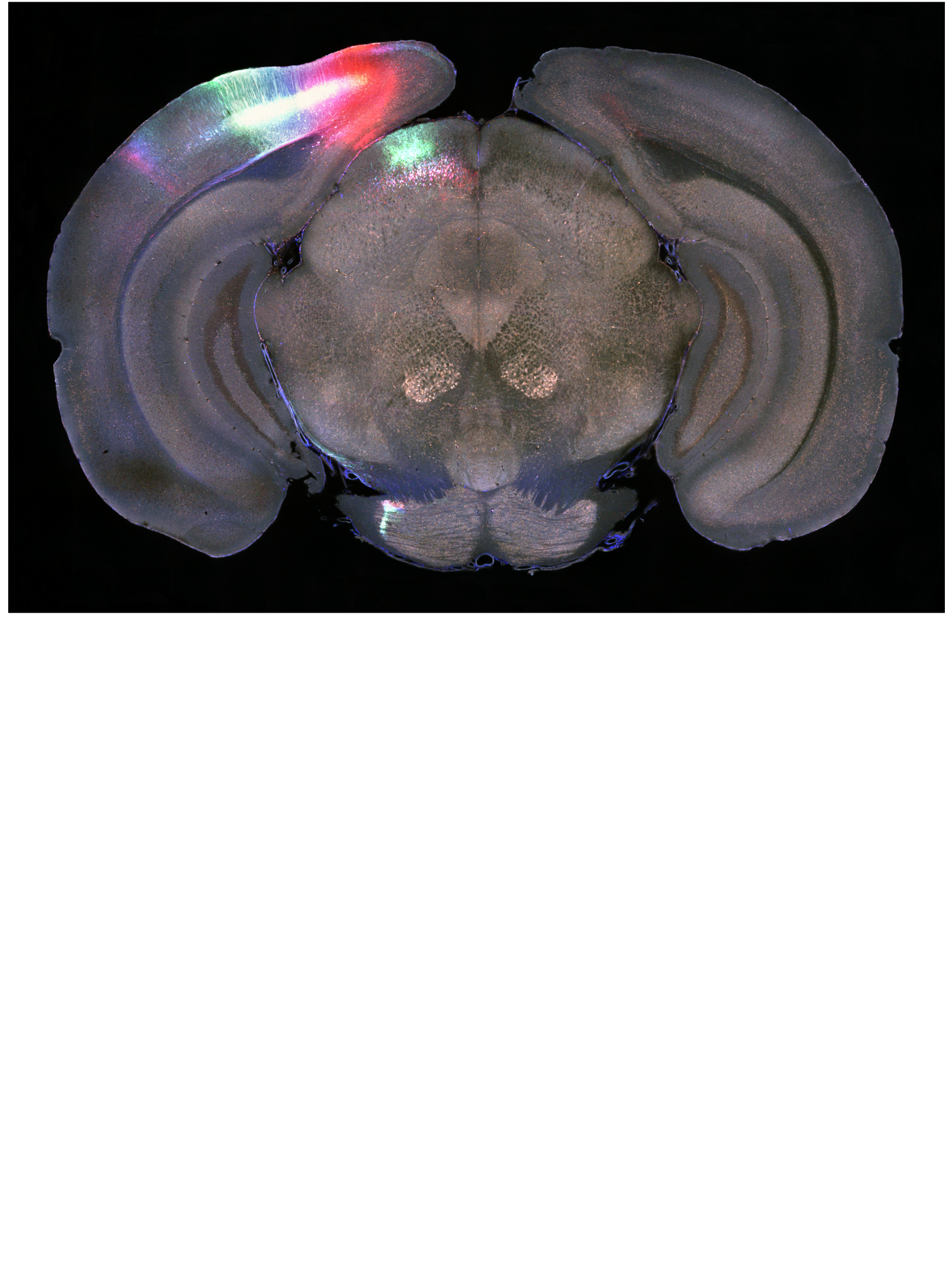
Viral tracing in mice
cFos-staining experiments (experimental support)
Maybe others?
Serial two-photon tomography
Light sheet fluorescence microscopy
cellfinder input data
cellfinder input data
cellfinder input data
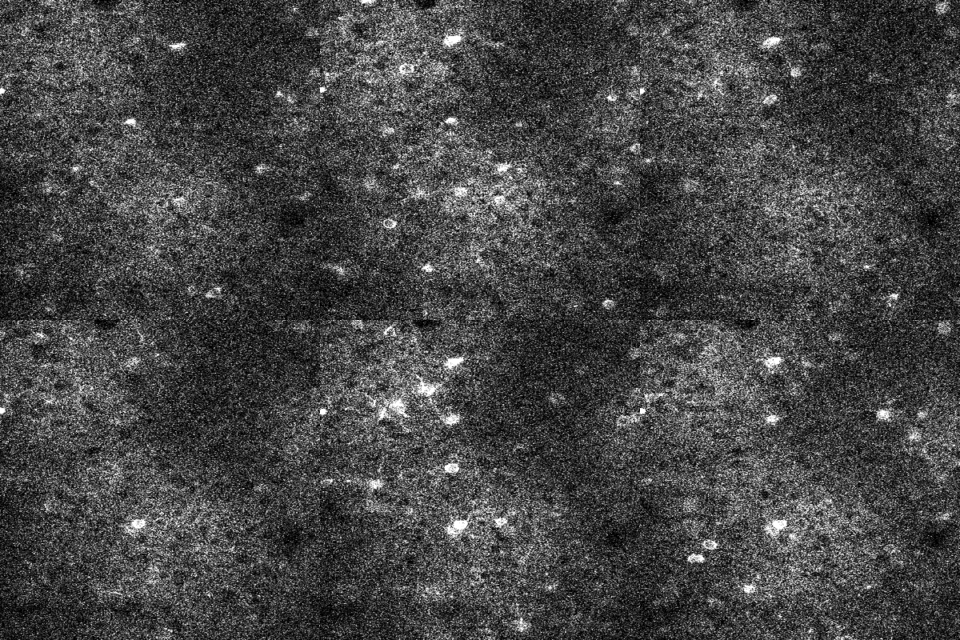
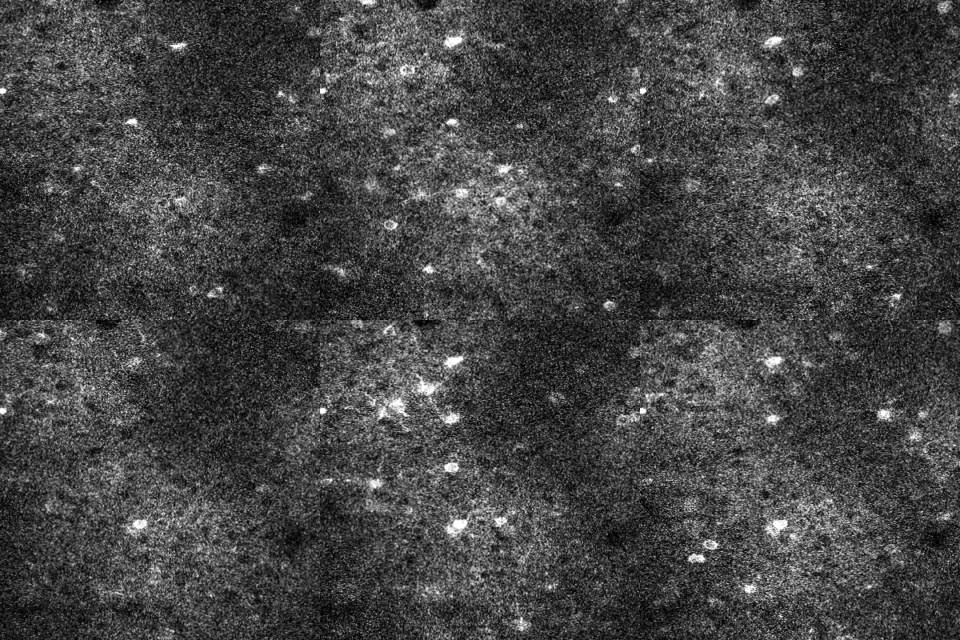
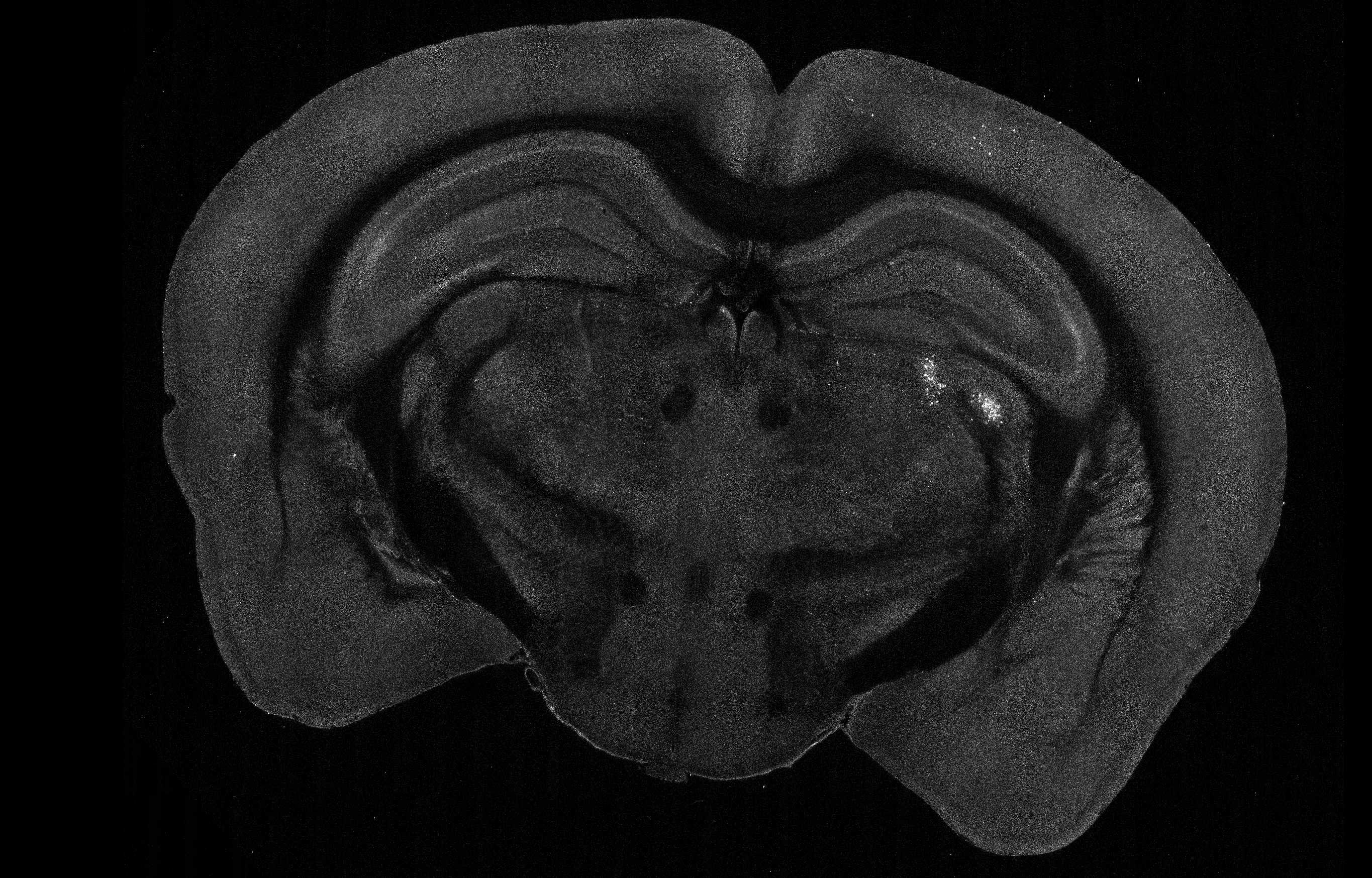
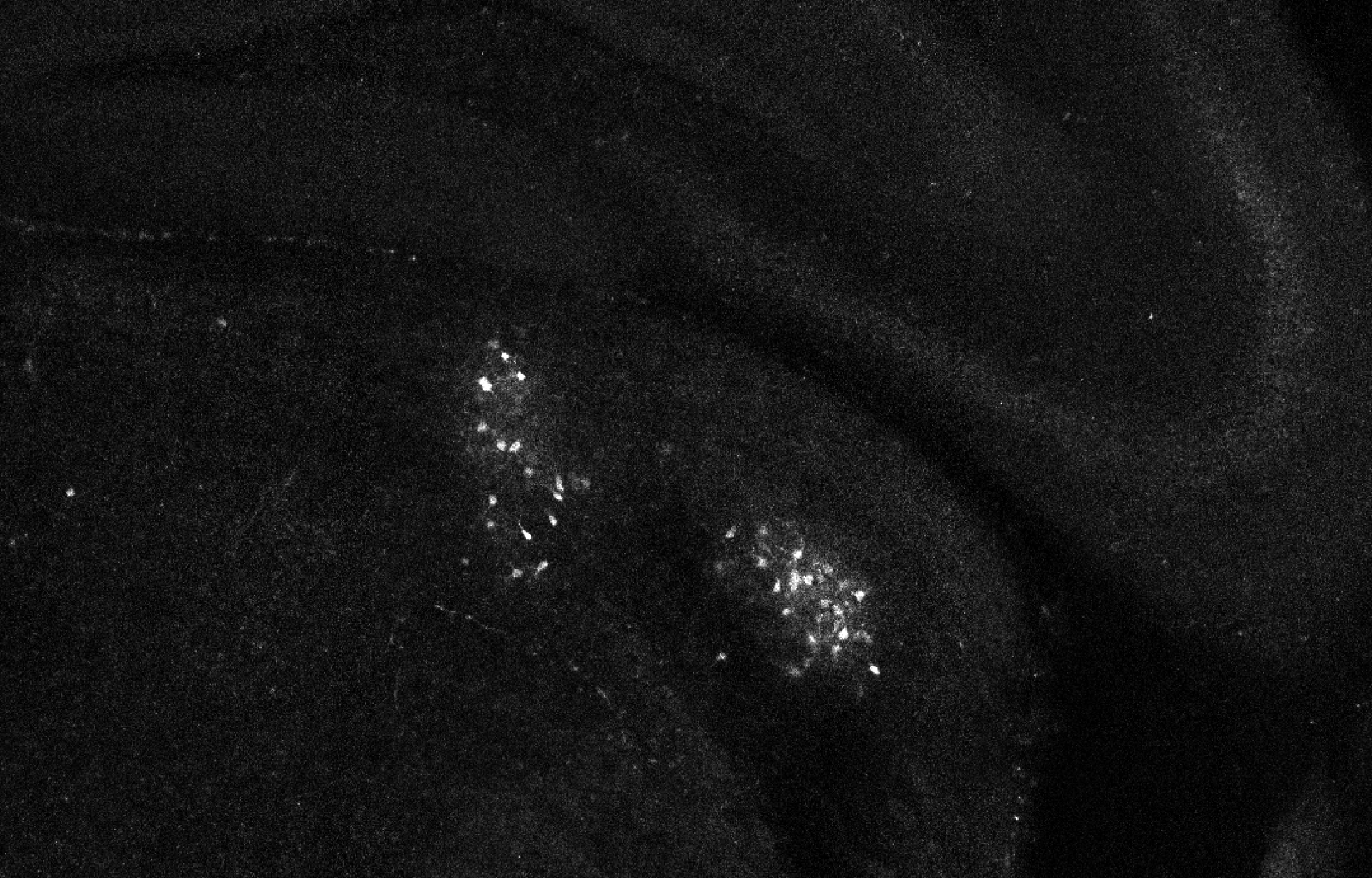
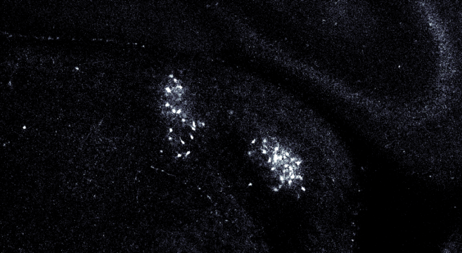
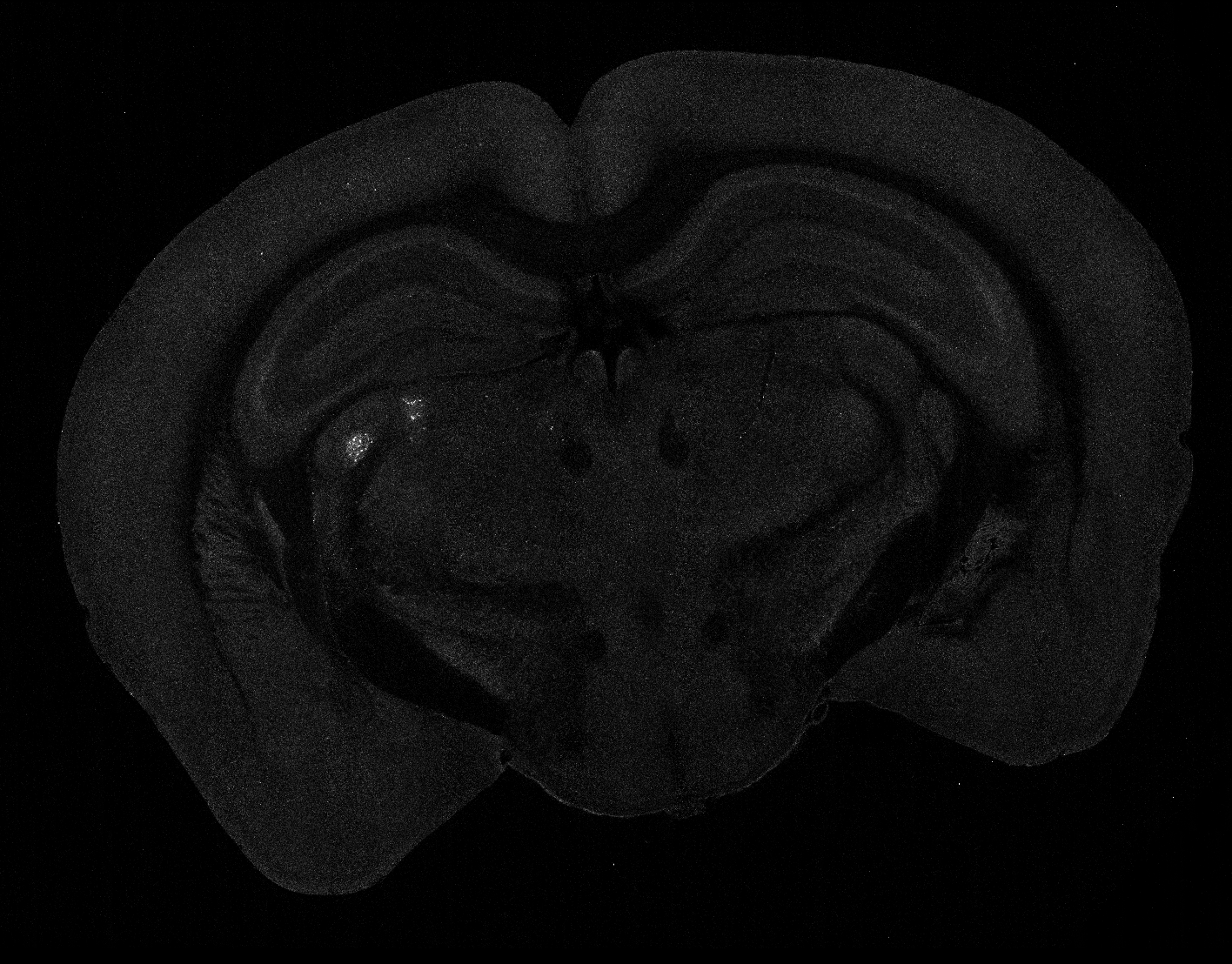
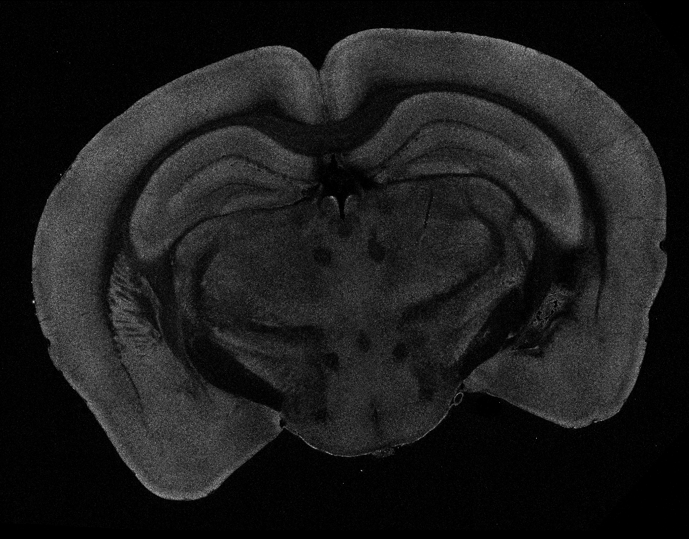
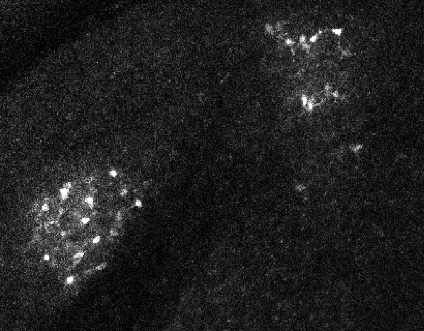
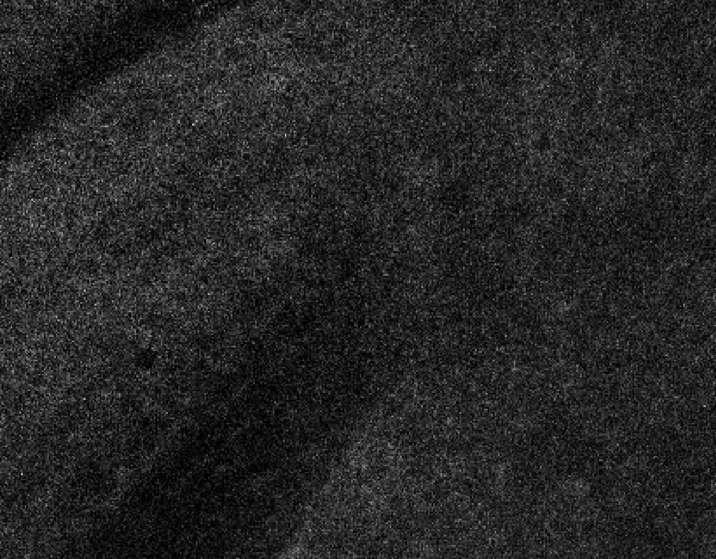
Whole brain microscopy, two channels
signal
background
cellfinder input data
Whole brain microscopy, two channels
signal
background
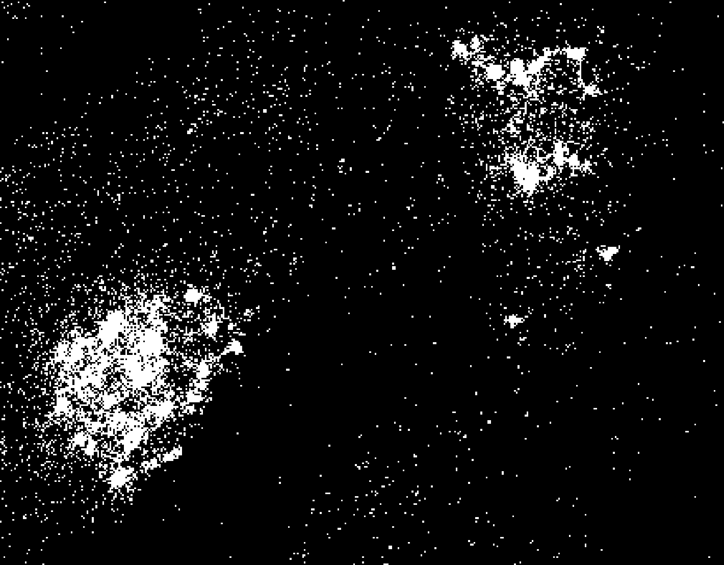
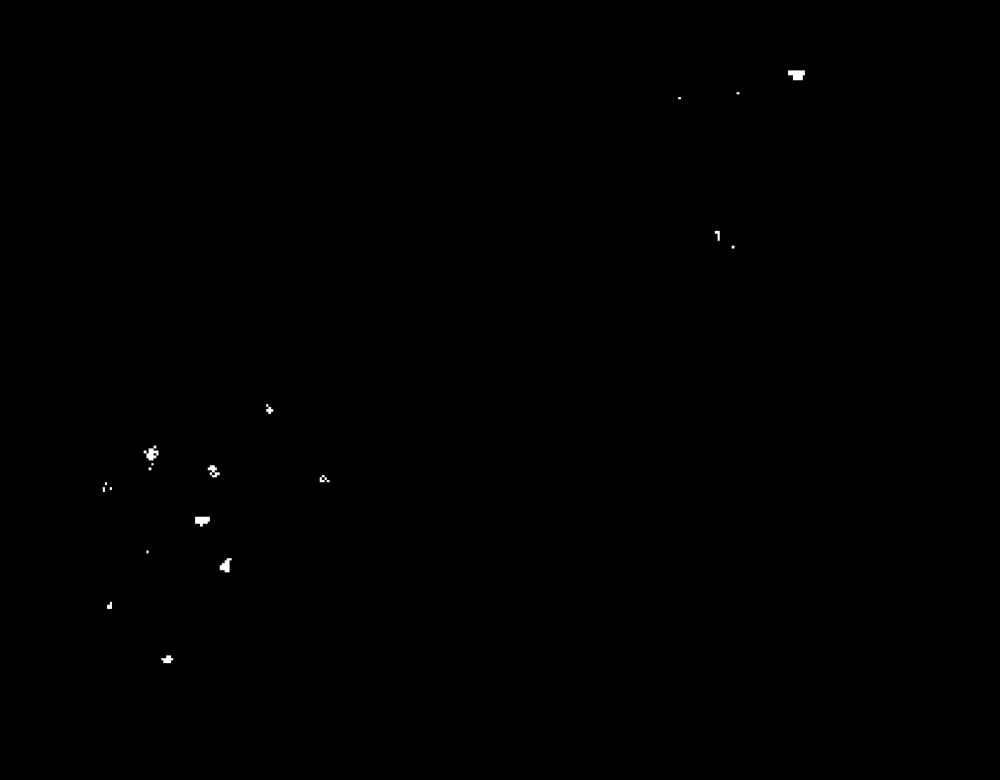
Why is 3D cell detection hard?
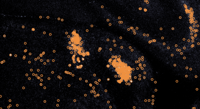
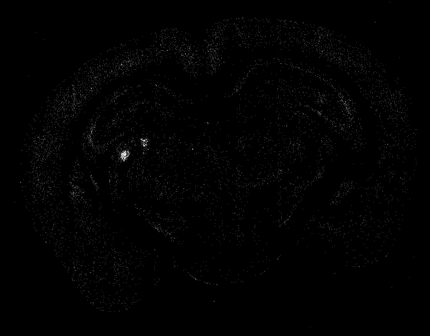
Classical image processing lacks sweet spot in noisy 3d microscopy.
Low threshold (2’000)
High threshold (10’000)
Why is 3D cell detection hard?
Classical image processing lacks sweet spot in noisy 3d microscopy.
Low threshold (2’000)
High threshold (10’000)
Why is 3D cell detection hard?
Pure machine-learning based methods are slow on such large data (~100GB per channel)
cellfinder strategy
Best of both worlds
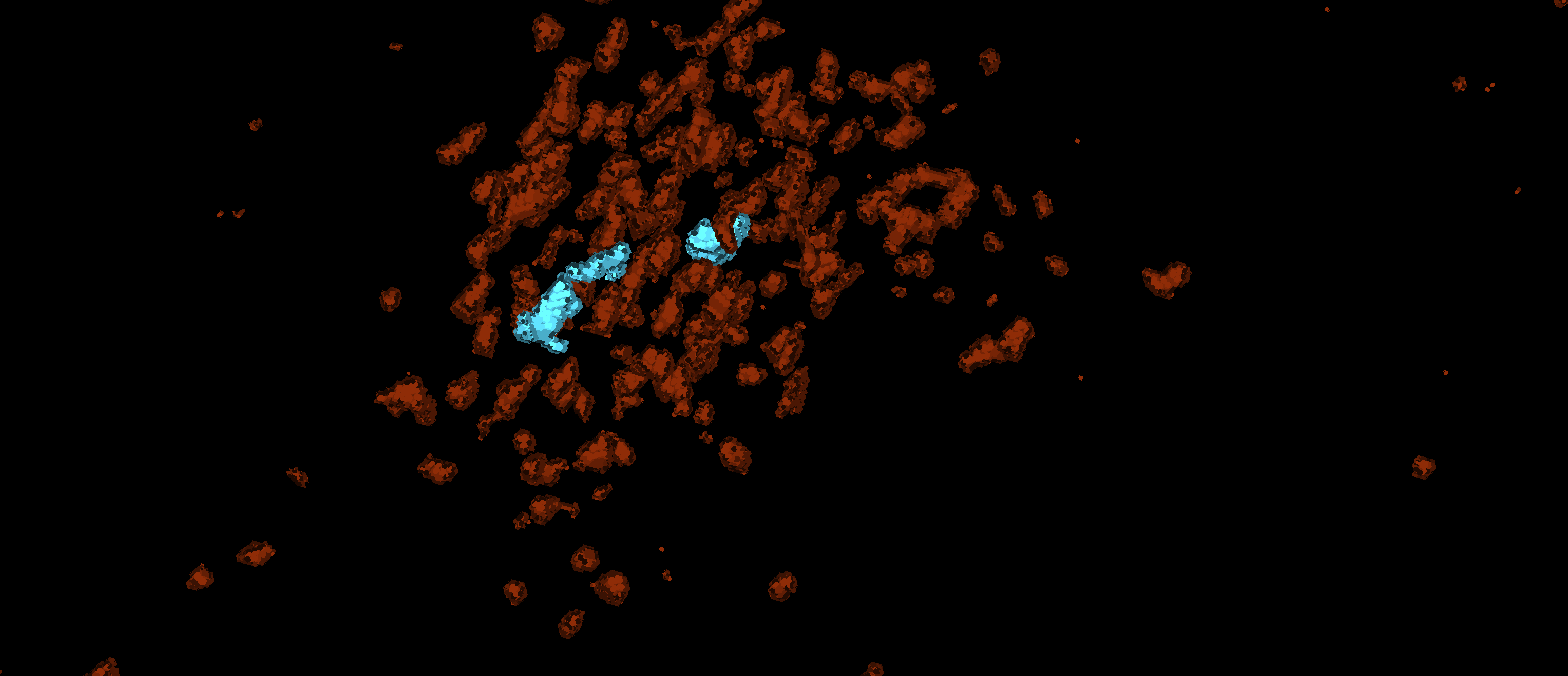
Select too many possible cells: “candidates”
Use machine-learning to classify candidates
binary classification: cell/not cell
needs curation and re-training
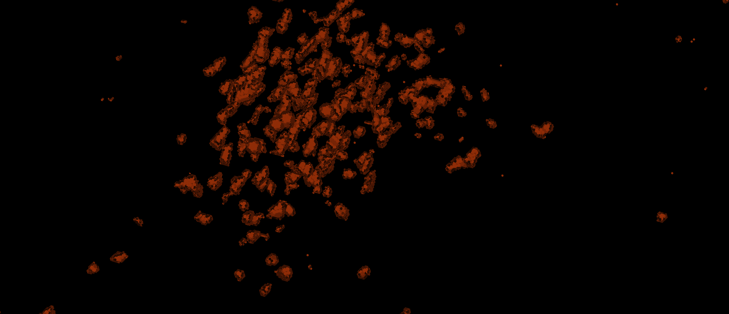
Cell candidate detction
Christian Niedwork Charly Rousseau Adam Tyson
Cell candidate detction
Christian Niedwork Charly Rousseau Adam Tyson
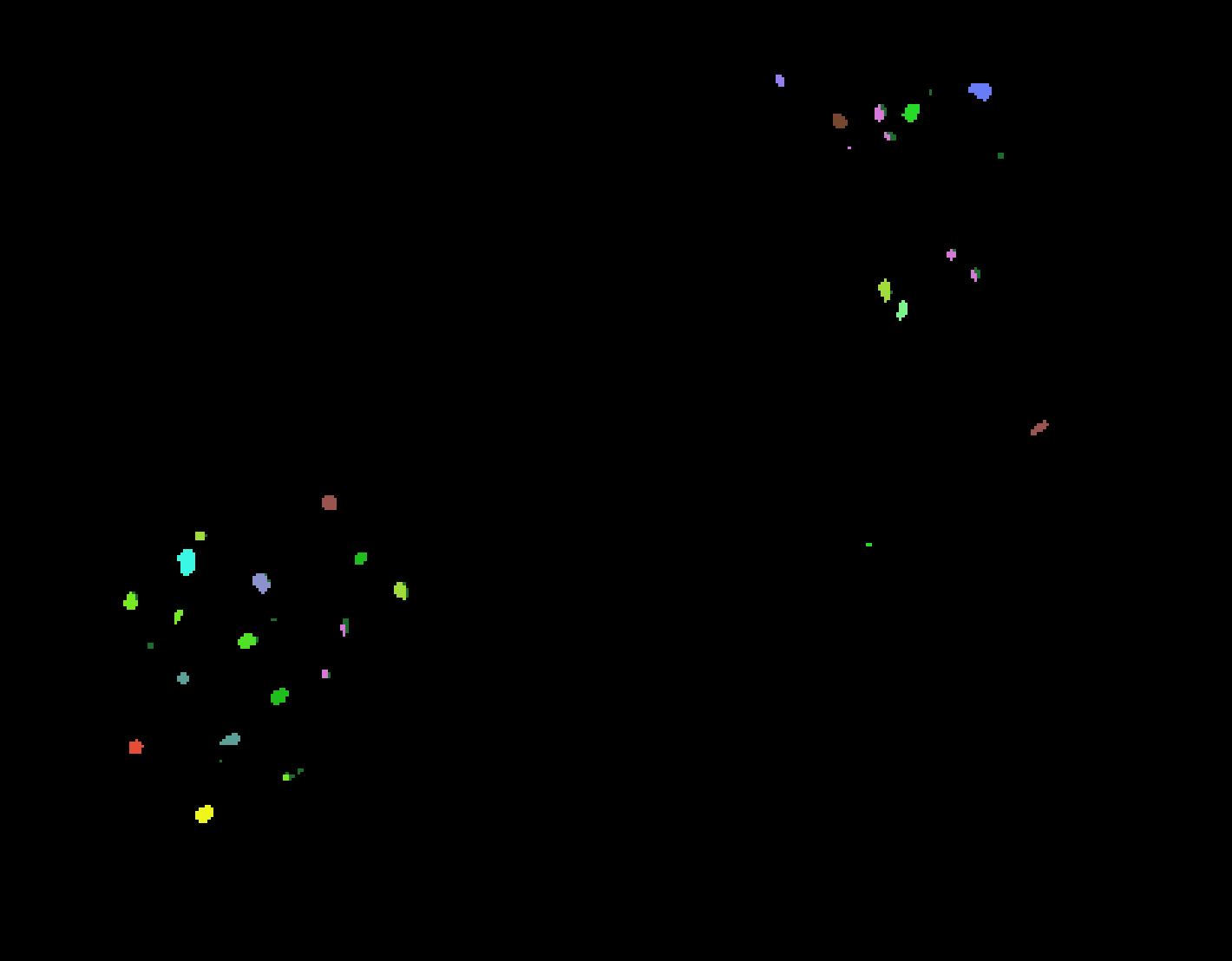
Cell candidate classification
Christian Niedwork Charly Rousseau Adam Tyson
Cellfinder high-level user workflow
%%{init: {'theme': 'default', 'flowchart': {'curve': 'basis'}}}%%
flowchart LR
    A[1. Detect<br/>Candidates] --> B[2. Classify<br/>Candidates]
    B --> C[3. Curate<br/>Candidates]
    C --> D[4. Retrain<br/>Model]
    D --> B
    B -.->|Further Analysis & Visualisation| E[ ]
    style E fill:transparent,stroke:transparent
    D ~~~ E
A series of image filters on the signal channel only
2D filter
3D filter
Structure splitting
2D filter
1. (Clip to reserve 2 values)
2. Keep bright enought tiles
3. Enhance peaks
a) median filter
b) gaussian filter
c) laplacian filter
4. Threshold
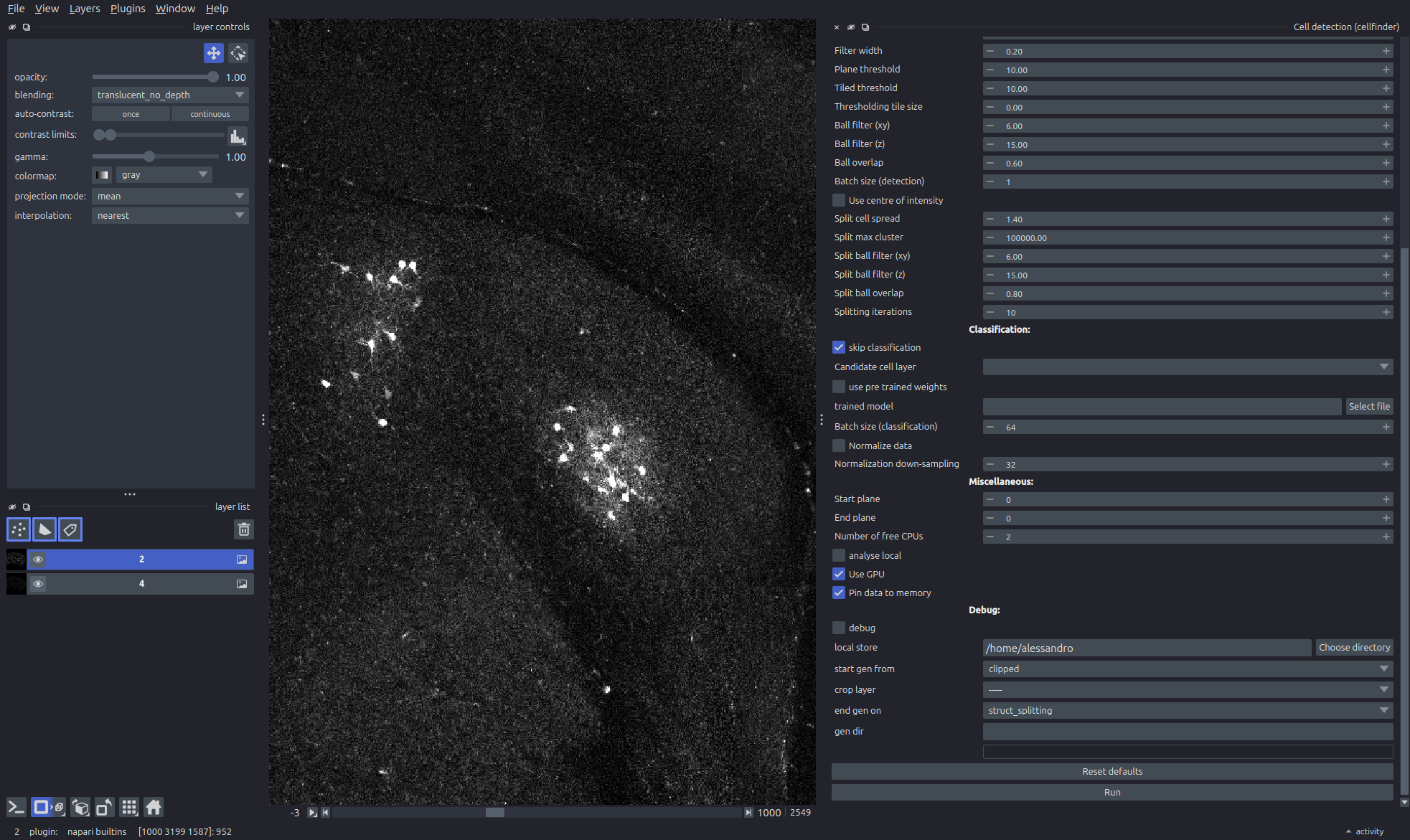
2D Filtering parameters
Parameter
Default
Description
log_sigma_size
0.2
Gaussian filter width (as a fraction of soma diameter) used during 2d in-plane Laplacian of Gaussian filtering.
soma_diameter
16
The expected in-plane (xy) soma diameter (microns).
n_sds_above_mean_thresh
10
Per-plane intensity threshold (the number of standard deviations above the mean) of the filtered 2d planes used to mark pixels as foreground or background.
3d filter + structure splitting
1. Looks at sphere (ellipsoid) around each pixel
a) If sufficient pixels in the ellipsoid are bright, mark as part of candidate
2. If needed structure is big, split it into several.
3. Compute and return centres of structures
Structure splitting in 3D
3D Filtering parameters
Parameter
Default
Description
ball_xy_size
6
3d filter’s in-plane (xy) filter ball size (microns).
ball_z_size
15
3d filter’s axial (z) filter ball size (microns).
ball_overlap_fraction
0.6
3d filter’s fraction of the ball filter needed to be filled by foreground voxels, centered on a voxel, to retain the voxel.
Splitting parameters
Parameter
Default
Description
split_ball_xy_size
6
Similar to ball_xy_size, except the value to use for the 3d filter during cluster splitting.
split_ball_z_size
15
Similar to ball_z_size, except the value to use for the 3d filter during cluster splitting.
split_ball_overlap_fraction
0.8
Similar to ball_overlap_fraction, except the value to use for the 3d filter during cluster splitting.
n_splitting_iter
10
The number of iterations to run the 3d filtering on a cluster. Each iteration reduces the cluster size by the voxels not retained in the previous iteration.
soma_spread_factor
1.4
Cell spread factor for determining the largest cell volume before splitting up cell clusters. Structures with spherical volume of diameter soma_spread_factor * soma_diameter or less will not be split.
max_cluster_size
100_000
Largest detected cell cluster (in cubic um) where splitting should be attempted. Clusters above this size will be labeled as artifacts.
Candidate coordinates
Store the average coordinate of each candidate.
Performance-related parameters
Parameter
Default
Description
batch_size
None (1 on GPU, 4 on CPU)
The number of planes of the original data volume to process at once. The GPU/CPU memory must be able to contain this many planes for all the filters. For performance-critical applications, tune to maximize memory usage without running out. Check your GPU/CPU memory to verify it’s not full.
torch_device
None
The device on which to run the computation. If not specified (None), “cuda” will be used if a GPU is available, otherwise “cpu”. You can also manually specify “cuda” or “cpu”.
pin_memory
False
Pins data to be sent to the GPU to the CPU memory. This allows faster GPU data speeds, but can only be used if the data used by the GPU can stay in the CPU RAM while the GPU uses it. I.e. there’s enough RAM. Otherwise, if there’s a risk of the RAM being paged, it shouldn’t be used. Defaults to False.
n_free_cpus
2
How many CPU cores to leave free.
Classification
Assumption: noise is bright in both channels, signal is bright only in one channel.
signal
background
Classification
Default model, use as starting point for retraining.
ResNet, trained on…
~100’000 manual annotations
50,653 cells
56,902 non-cells
from 5 brains
Classification parameters
Parameter
Default
Description
cube_width
50
The width of the data cube centered on the cell used for classification.
cube_height
50
The height of the data cube centered on the cell used for classification.
cube_depth
20
The depth of the data cube centered on the cell used for classification.
network_depth
50
The network depth to use during classification.
normalize_channels
False
If True, the signal and background data will be each normalized to a mean of zero and standard deviation of 1 before classification.
normalization_n_sampling_planes
50
If normalize_channels is True, the data arrays will be down-sampled in the first axis to use approximately this many planes – equally spaced, before calculating their mean/std. E.g. a value of 50 for a dataset of 200 planes means every fourth plane will be used.
max_workers
3
The max number of sub-processes to use for data loading / processing during classification.
Stretch exercise: Fine-tune detection parameters on your data with this experimental napari plugin addition, in a new environment.
Cellfinder high-level workflow
%%{init: {'theme': 'default', 'flowchart': {'curve': 'basis'}}}%%
flowchart LR
    A[1. Detect<br/>Candidates] --> B[2. Classify<br/>Candidates]
    B --> C[3. Curate<br/>Candidates]
    C --> D[4. Retrain<br/>Model]
    D --> B
    B -.->|Further Analysis & Visualisation| E[ ]
    style E fill:transparent,stroke:transparent
    D ~~~ E
Curation and retraining
Suggested strategy
spend hours, not days curating
iterate fast: curate, retrain, classify and repeat
curated balanced data (equal number of cells/not cells)
Reminder: only candidate cells will be classified
Retraining parameters
Parameter
Default
Description
trained_model
-
Path to the trained model
network_depth
50
Resnet depth (based on He et al. (2015)
learning_rate
0.0001
Learning rate for training the model
test_fraction
0.1
Fraction of training data to use for validation
epochs
100
Number of training epochs
no_augment
False
If True, don’t apply data augmentation
augment_likelihood
0.9
Value [0, 1] with the probability of a data item being augmented. I.e. 0.9 means 90%% of the data will have been augmented.
lr_schedule
()
If not empty, the list of epochs when to multiply the current learning rate by the lr_multiplier. E.g. if it’s [10, 25], we start with a learning rate of 0.001, and lr_multiplier is 0.1, then the LR will be 0.001 for epochs 0-9, 0.0001 for 10-24, and 0.0001 for epoch 25 and beyond.
lr_multiplier
0.1
The multiplier by which to multiply the previous learning rate at the epochs listed in lr_schedule.
augment_likelihood
0.9
Value [0, 1] with the probability of a data item being augmented. I.e. 0.9 means 90%% of the data will have been augmented.
normalize_channels
False
Normalize the training data to the mean/std of the datasets from which the cubes came from.
Retraining parameters
Parameter
Default
Description
continue_training
False
Continue training from an existing trained model. If no model or model weights are specified, this will continue from the included model.
batch_size
16
Training batch size
tensorboard
False
Log to output_directory/tensorboard
max_workers
3
Maximum number of worker processes to use to load data
pin_memory
True
Pins data to be sent to the GPU to the CPU memory. This allows faster GPU data speeds, but can only be used if the data used by the GPU can stay in the CPU RAM while the GPU uses it. I.e. there’s enough RAM. Otherwise, if there’s a risk of the RAM being paged, it shouldn’t be used.






 /
/ 


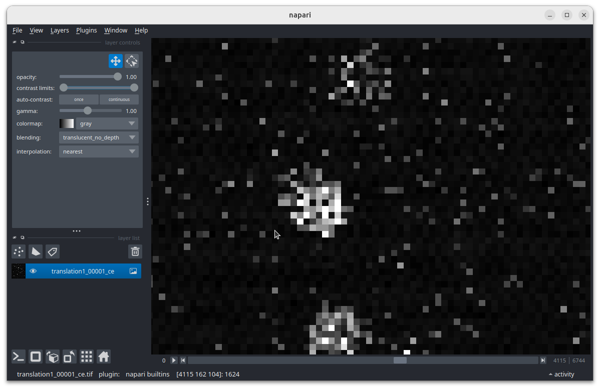
 and run: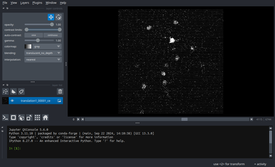
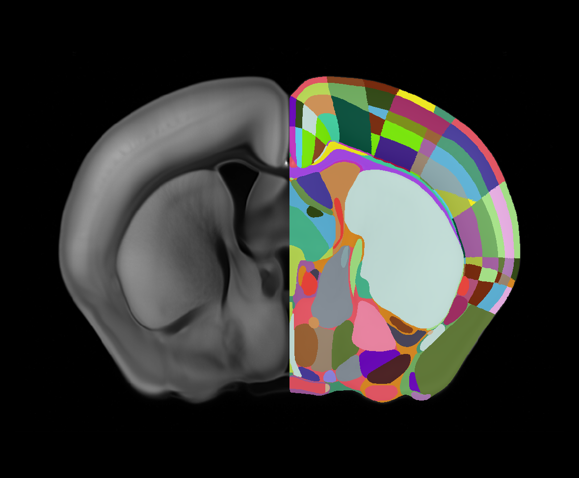
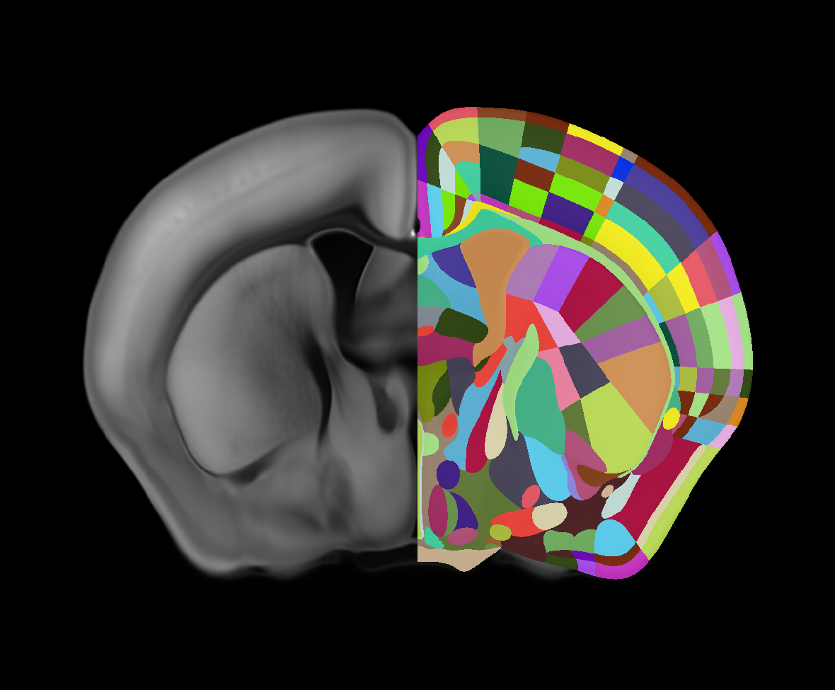
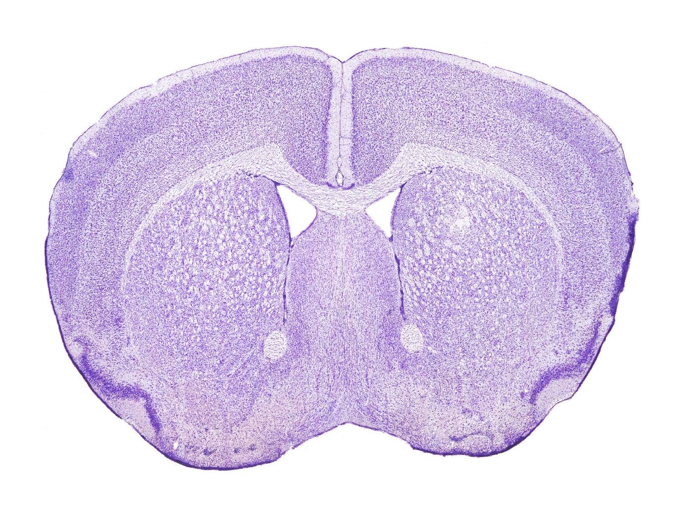 Template
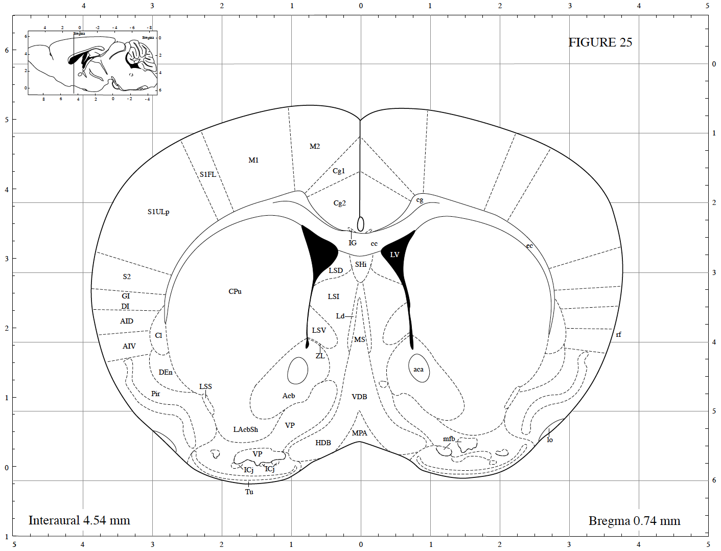 Annotation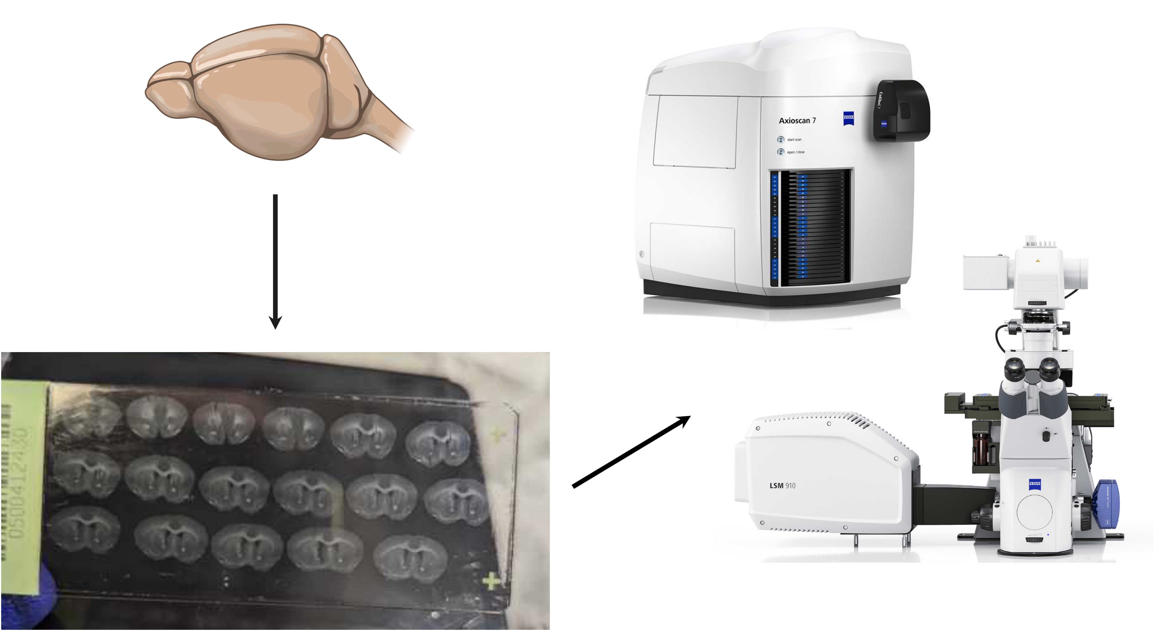
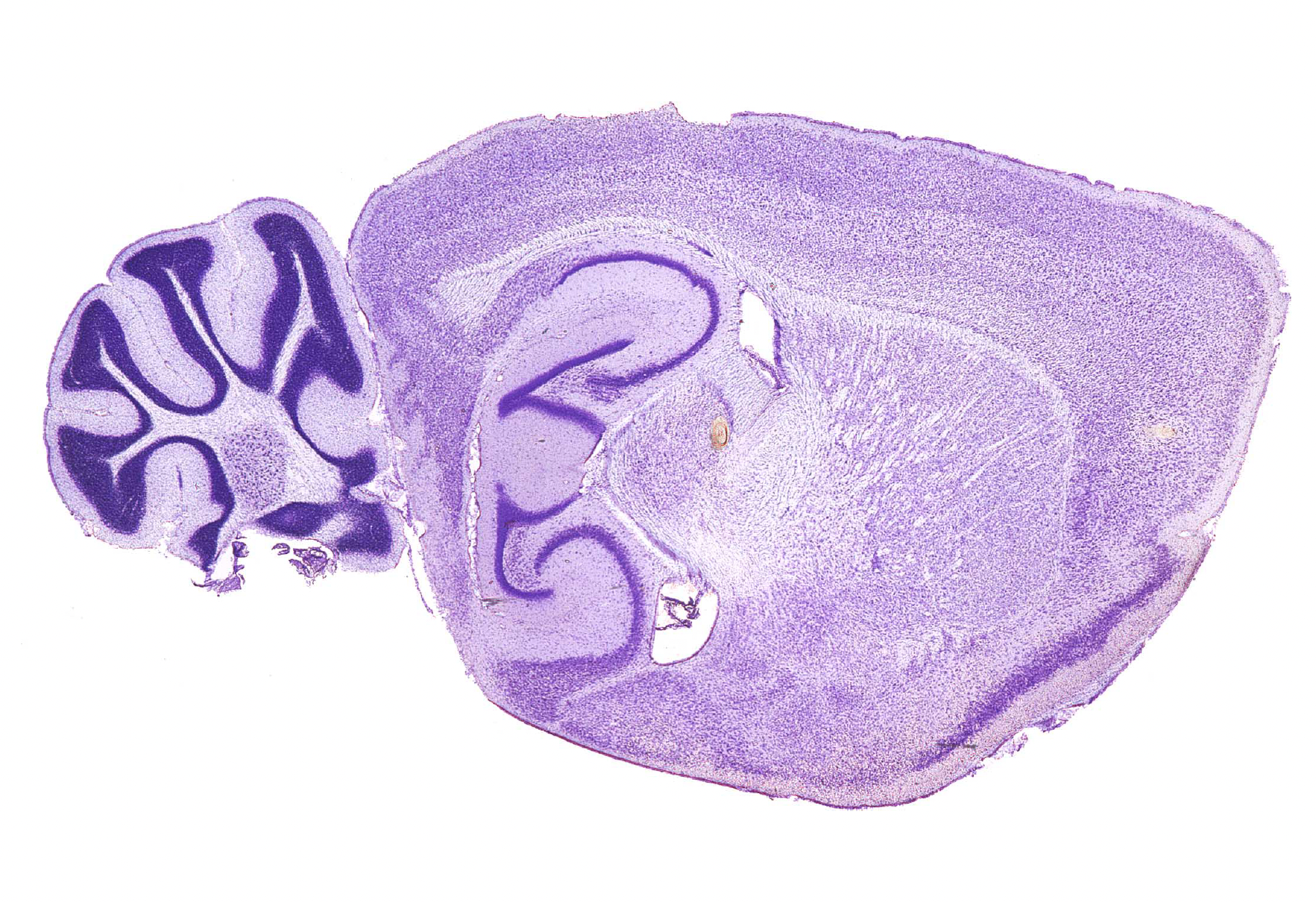
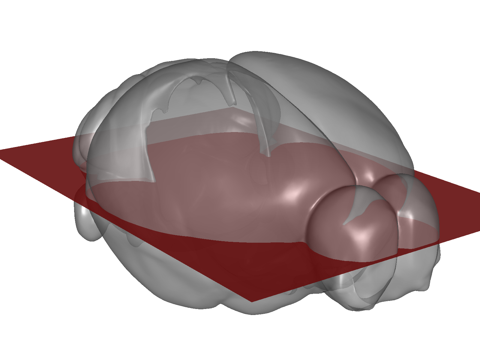
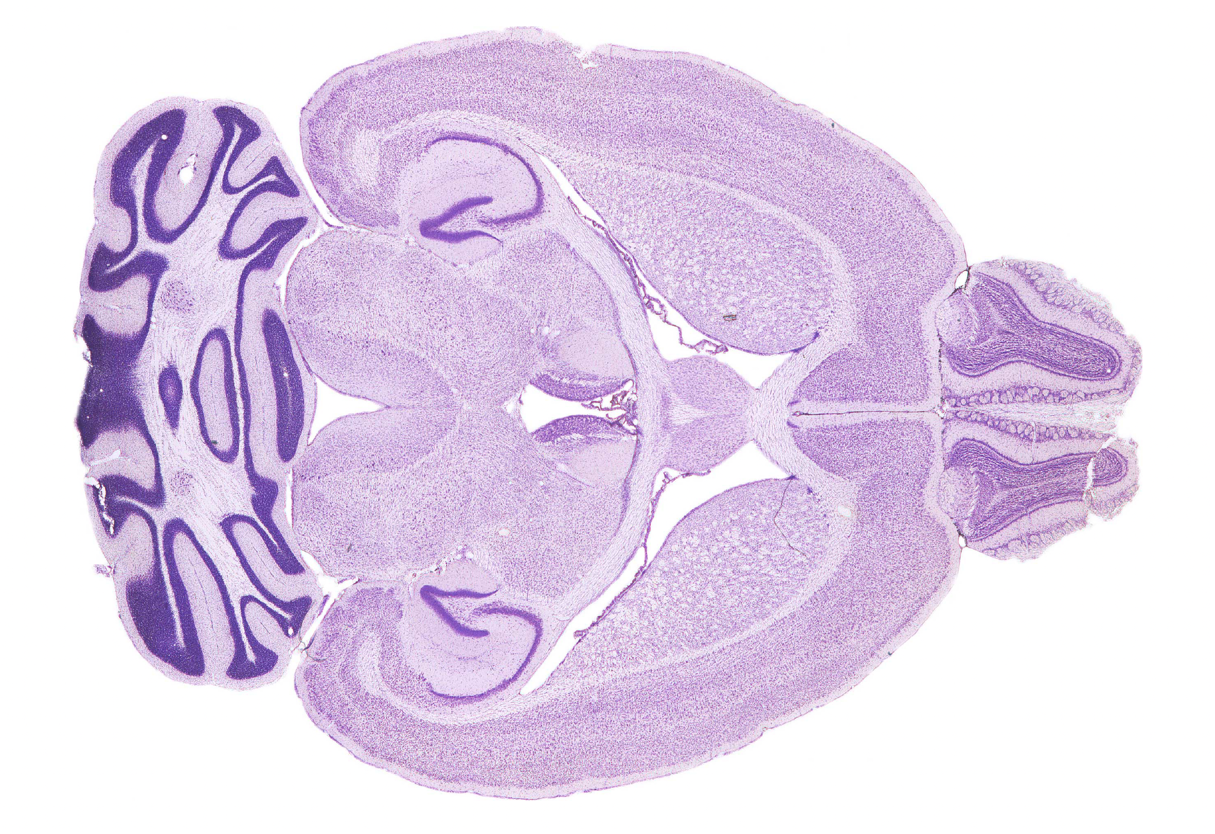
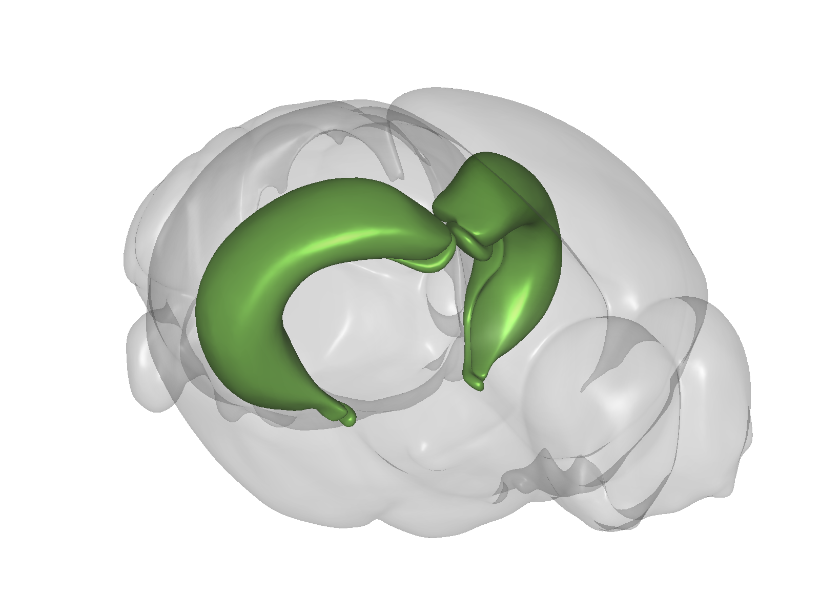



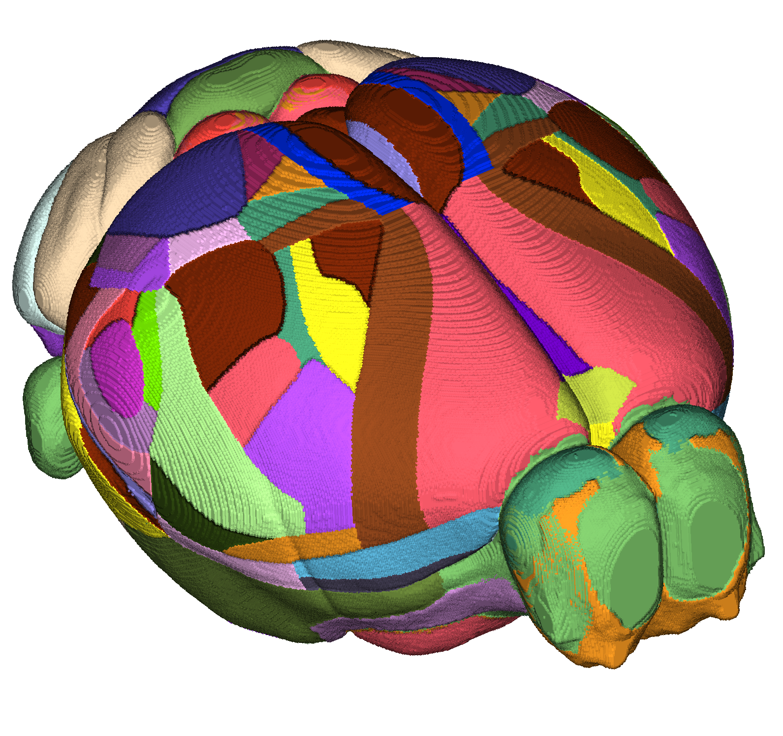


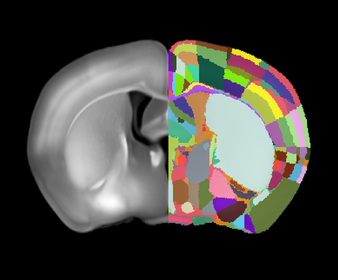
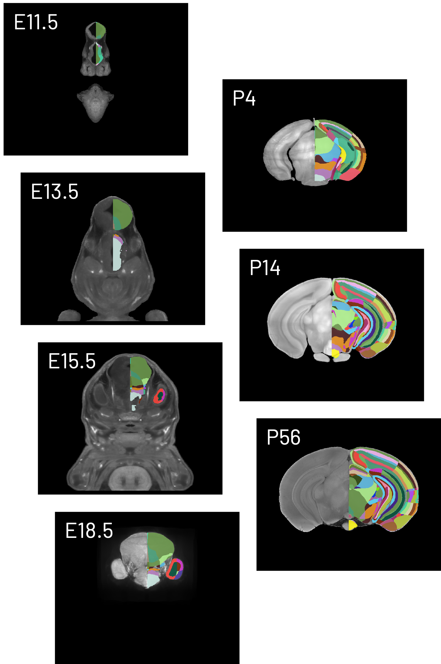 DevCCF
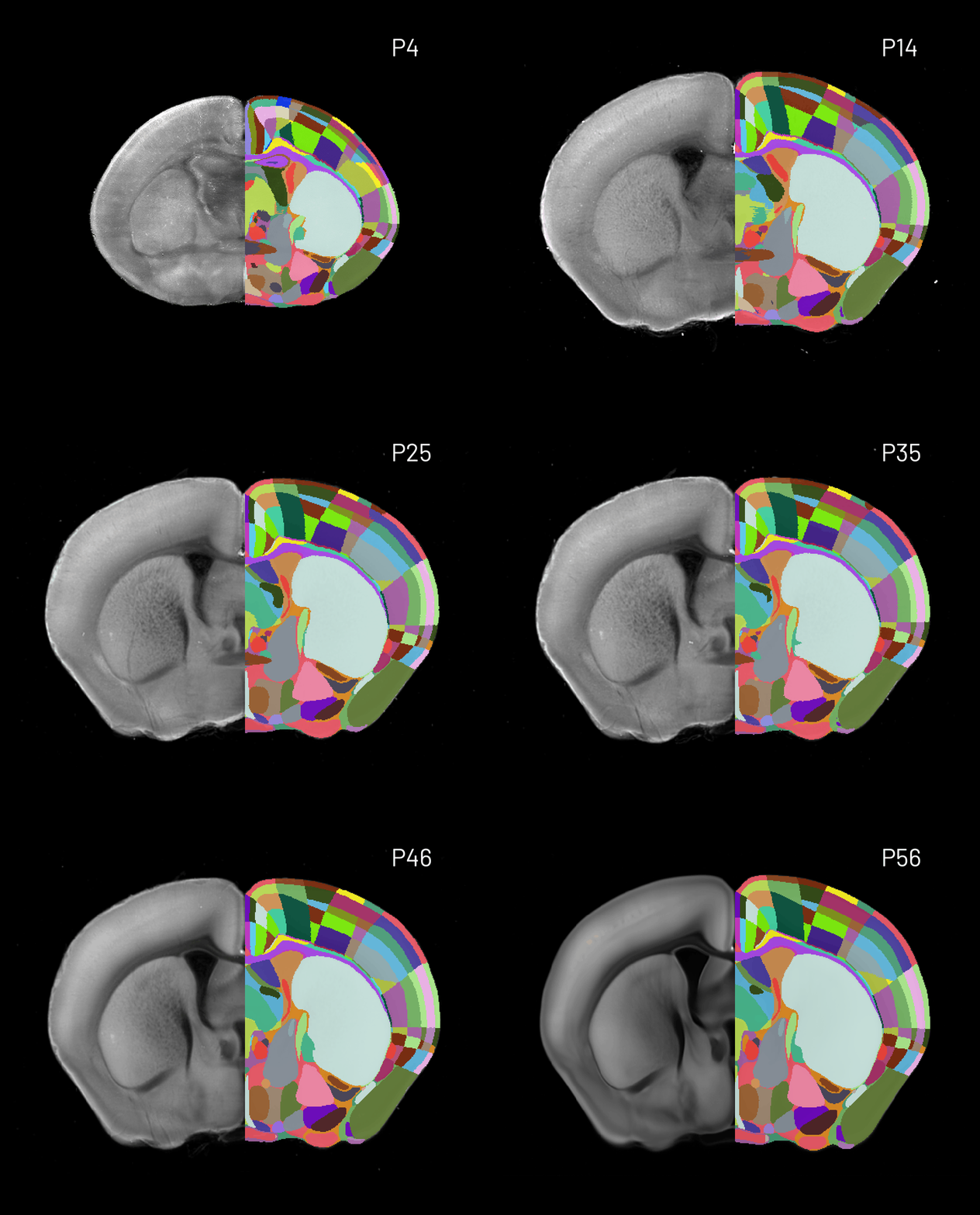 Developmental Mouse Brain Atlas


 signal
 background
 signal
 background
 Low threshold (2’000)
 High threshold (10’000)
 Low threshold (2’000)
 High threshold (10’000)