Note
Go to the end to download the full example code.
Interacting with cloud atlas data through Python#
This example demonstrates how to calculate the volume of the retrosplenial area in the Allen mouse brain atlas at 25um resolution. It does so avoiding use of BrainGlobe tools, and using minimal other dependencies. It is intended to showcase the use of atlas data directly.
This tutorial will guide through the steps needed to extract the volume of the retrosplenial area (RSP) in the Allen Mouse Brain Atlas, programmatically - but without using BrainGlobe. To do this, we need some preliminary knowledge about how BrainGlobe atlases such as this are structured under the hood:
the annotation image is stored as an OME-Zarr <https://ngff.openmicroscopy.org/#next-generation-file-formats-ngff-ome-zarr>.
the region metadata (e.g. each region’s id, name, acronym and parent) are stored in a comma separated (csv) file
these files (and other atlas files, like the template) are stored on AWS
To compute the volume of RSP we will therefore
access the terminologies file
determine the id of the RSP region and all its children from the terminologies file
access the annotation file
count how many pixels in the annotation file correspond to any of the ids
convert the pixels to cubic millimeters
Now the conceptual part is covered, let’s dive into the code:
We start by importing some Python libraries that we will need
import dask.array as da
import ngff_zarr as nz
import numpy as np
import pandas as pd
from matplotlib import pyplot as plt
from matplotlib import colormaps as cm
Next, we use pandas to access the terminologies files using its S3 URI.
s3_bucket_stub = "s3://brainglobe/atlas/{}"
annotation_uri = s3_bucket_stub.format("annotation-sets/allen_mouse-annotation/1_2/annotation.ome.zarr")
terminologies_uri = s3_bucket_stub.format("terminologies/allen_mouse-terminology/1_2/terminology.csv")

terminologies_df = pd.read_csv(terminologies_uri, storage_options={"anon": True})
By printing the dataframe, we can observe that the terminologies file contains one row per region, with the first column (index 0) containing the region abbreviation, and the second column (index 1) containing the region ID:
terminologies_df.head()
We know that all child regions of RSP have an abbreviation starting with “RSP”, which we can use to identify our IDs of interest and store them in a list called rsp_ids.
terminologies_filtered = terminologies_df[terminologies_df["abbreviation"].str.startswith("RSP")]

rsp_ids = terminologies_filtered["annotation_value"].tolist()
Equipped with this information, we can now access the annotations file for the atlas. Annotation files are stored in an OME-zarr file in the cloud.
annotations = nz.from_ngff_zarr(annotation_uri, storage_options={"anon": True})

print(annotations.metadata)
Metadata(axes=[Axis(name='z', type='space', unit='millimeter', orientation={'type': 'anatomical', 'value': 'anterior-to-posterior'}), Axis(name='y', type='space', unit='millimeter', orientation={'type': 'anatomical', 'value': 'superior-to-inferior'}), Axis(name='x', type='space', unit='millimeter', orientation={'type': 'anatomical', 'value': 'right-to-left'})], datasets=[Dataset(path='0', coordinateTransformations=[Scale(scale=[0.01, 0.01, 0.01], type='scale')]), Dataset(path='1', coordinateTransformations=[Scale(scale=[0.025, 0.025, 0.025], type='scale')]), Dataset(path='2', coordinateTransformations=[Scale(scale=[0.05, 0.05, 0.05], type='scale')]), Dataset(path='3', coordinateTransformations=[Scale(scale=[0.1, 0.1, 0.1], type='scale')])], coordinateTransformations=None, omero=None, name='/', type=None, metadata=None)
We can see from the metadata that the zarr contains multiple resolution levels (a pyramid). For this tutorial, we will use the highest resolution level (level 0).
pyramid_level = 0
annotation_image = annotations.images[pyramid_level]

print(annotation_image)
NgffImage(data=dask.array<from-zarr, shape=(1320, 800, 1140), dtype=uint32, chunksize=(83, 100, 143), chunktype=numpy.ndarray>, dims=('z', 'y', 'x'), scale={'z': 0.01, 'y': 0.01, 'x': 0.01}, translation={'z': 0.0, 'y': 0.0, 'x': 0.0}, name='/', axes_units={'z': 'millimeter', 'y': 'millimeter', 'x': 'millimeter'}, axes_orientations=None, channel_names=None, channel_colors=None, computed_callbacks=[])
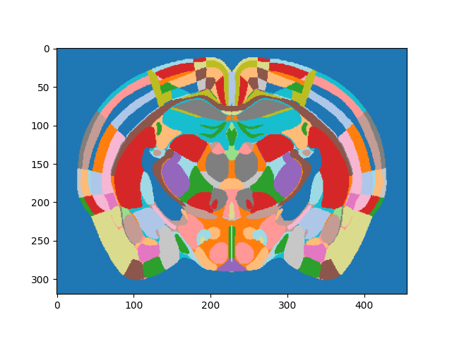
By plotting a slice of the array contents, we can see the various regions encoded by integer values:
# Get the middle section and plot
middle_section = annotation_image.data.shape[0] // 2

# Create a cyclic colormap due to the high values in the Allen atlas
N = 512
colors = cm.get_cmap('tab20').resampled(N)
lut = colors(np.arange(N))

# Map label image to lookup table and plot
plt.imshow(lut[annotation_image.data[middle_section,:,:] % N])
<matplotlib.image.AxesImage object at 0x7ff1bd018dd0>
Combining the annotation data with our RSP IDs allows us to calculate the volume of the RSP, which we finally print. This reaches the goal of this tutorial.
print(annotation_image.scale)
print(annotation_image.axes_units)

num_pixels = da.isin(annotation_image.data[:], rsp_ids).sum().compute()
pixel_size_list = list(annotation_image.scale.values())
pixel_volume = pixel_size_list[0] * pixel_size_list[1] * pixel_size_list[2]  # in cubic millimeters

print(f"RSP has volume of around {np.round(num_pixels*pixel_volume)} cubic millimeters")
{'z': 0.01, 'y': 0.01, 'x': 0.01}
{'z': 'millimeter', 'y': 'millimeter', 'x': 'millimeter'}
RSP has volume of around 11.0 cubic millimeters
In conclusion, this tutorial shows how to programmatically access and process atlas data for the specific purpose of calculating a region volume. More generally, it also constitutes an example for BrainGlobe atlas data being used independently of the BrainGlobe software tools.
Total running time of the script: (1 minutes 0.937 seconds)